Here are the Code examples of this chapter. These pages are currently being updated over time (adding pictures, captions, and possibly further examples). Visit again soon for updates. Of course, the best way to use this page is together with the book for getting the explanations.

Figure 3.1 – A node with colors
\documentclass[tikz,border=10pt]{standalone}
\begin{document}
\begin{tikzpicture}
  \draw (4,2) node[draw, color=red, fill=yellow, text=blue] {TikZ};
\end{tikzpicture}
\end{document}
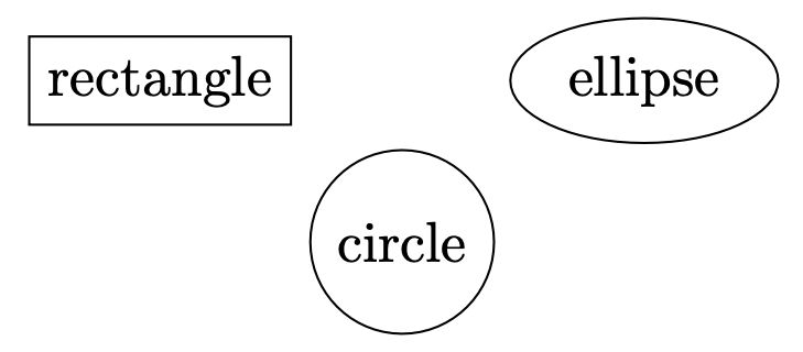
Figure 3.2 – Nodes with different shapes
\documentclass[tikz,border=10pt]{standalone}
\usetikzlibrary{shapes}
\begin{document}
\begin{tikzpicture}
  \node (r) at (0,1)   [draw, rectangle] {rectangle};
  \node (c) at (1.5,0) [draw, circle]    {circle};
  \node (e) at (3,1)   [draw, ellipse]   {ellipse};
\end{tikzpicture}
\end{document}
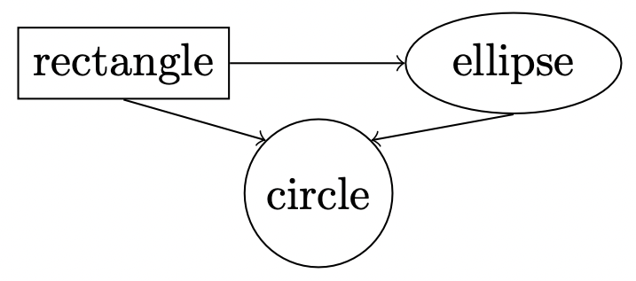
Figure 3.3 – Nodes with arrows
\documentclass[tikz,border=10pt]{standalone}
\usetikzlibrary{shapes}
\begin{document}
\begin{tikzpicture}
  \node (r) at (0,1)   [draw, rectangle] {rectangle};
  \node (c) at (1.5,0) [draw, circle]    {circle};
  \node (e) at (3,1)   [draw, ellipse]   {ellipse};
  \draw[->] (r.east)  -- (e.west);
  \draw[->] (r.south) -- (c.north west);
  \draw[->] (e.south) -- (c.north east);
\end{tikzpicture}
\end{document}

Figure 3.4 – Default anchor
\documentclass[tikz,border=10pt]{standalone}
\begin{document}
\begin{tikzpicture}
\draw[fill=red] (4,2) circle[radius=0.1];
\node at (4,2) [draw, rectangle] {rectangle};
\end{tikzpicture}
\end{document}

Figure 3.5 – Southwest anchor
\documentclass[tikz,border=10pt]{standalone}
\begin{document}
\begin{tikzpicture}
  \draw[fill=red] (4,2) circle[radius=0.1];
  \node at (4,2) [draw, rectangle, anchor=south west]
    {rectangle};
\end{tikzpicture}
\end{document}
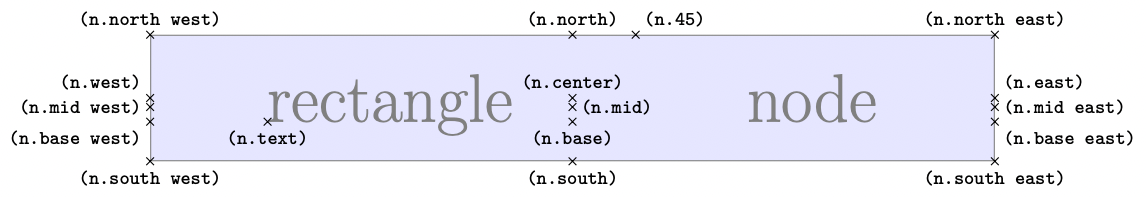
Figure 3.6 – Rectangle shape with anchors
\documentclass[tikz,border=5]{standalone}
\usetikzlibrary{positioning}
\tikzset{shape example/.style = {
    color=black!50, draw, fill=blue!10,
    inner xsep=1.5cm, inner ysep=0.5cm,
}}
\begin{document}
\Huge
\begin{tikzpicture}[node distance = 1mm]
  \node[name=n,shape=rectangle,shape example]
    {\Huge rectan\smash{g}le\hspace{3cm}node};
  \foreach \anchor/\placement in
    {center/above, text/below, 45/above right,
       mid/right, mid east/right, mid west/left,
       base/below, base east/below right, base west/below left,
       north/above, south/below, east/above right, west/above left,
       north east/above, south east/below, south west/below, north west/above}
      \draw[shift=(n.\anchor)] plot[mark=x] coordinates{(0,0)}
        node[\placement,label distance = 0mm,inner sep=3pt]
          {\scriptsize\texttt{(n.\anchor)}};
\end{tikzpicture}
\end{document}
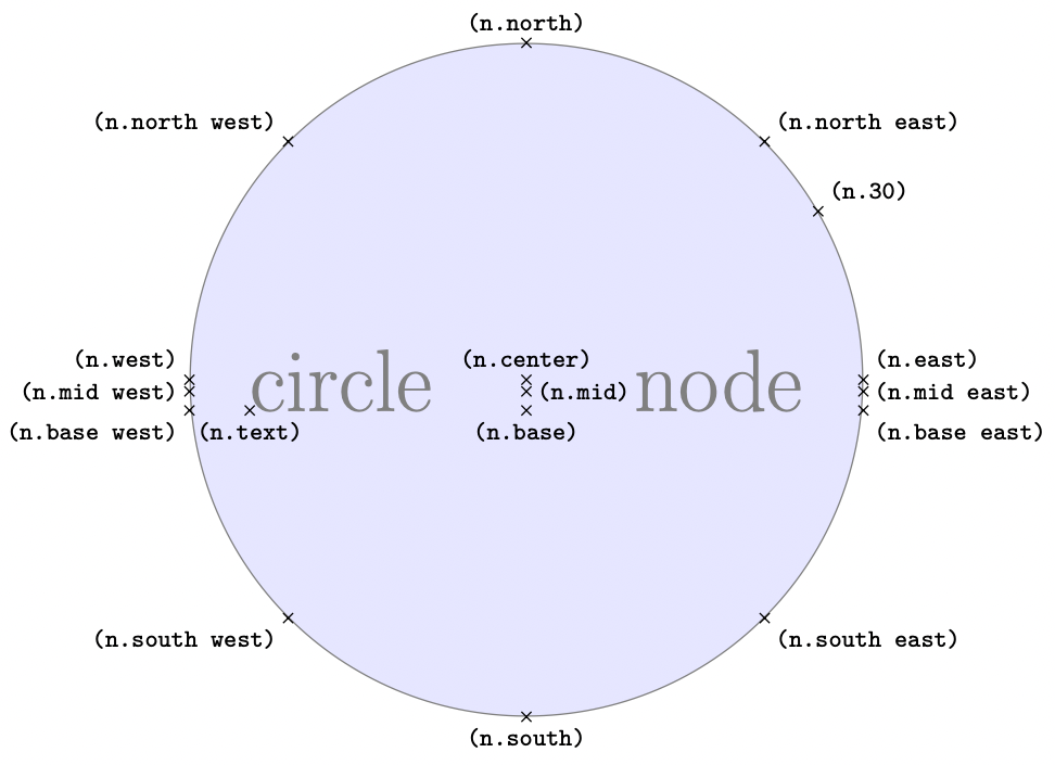
Figure 3.7 – Circle shape with anchors
\documentclass[tikz,border=5]{standalone}
\usetikzlibrary{positioning}
\tikzset{shape example/.style = {
    color=black!50, draw, fill=blue!10,
    inner xsep=0.5cm, inner ysep=0.5cm,
}}
\begin{document}
\Huge
\begin{tikzpicture}[node distance = 1mm]
  \node[name=n,shape=circle,shape example] {\Huge circle\hspace{2cm}node};
  \foreach \anchor/\placement in
    {center/above, text/below, 30/above right,
       mid/right, mid east/right, mid west/left,
       base/below, base east/below right, base west/below left,
       north/above, south/below, east/above right, west/above left,
       north east/above right, south east/below right, south west/below left,
         north west/above left}
      \draw[shift=(n.\anchor)] plot[mark=x] coordinates{(0,0)}
        node[\placement,label distance = 0mm,inner sep=3pt]
          {\scriptsize\texttt{(n.\anchor)}};
\end{tikzpicture}
\end{document}
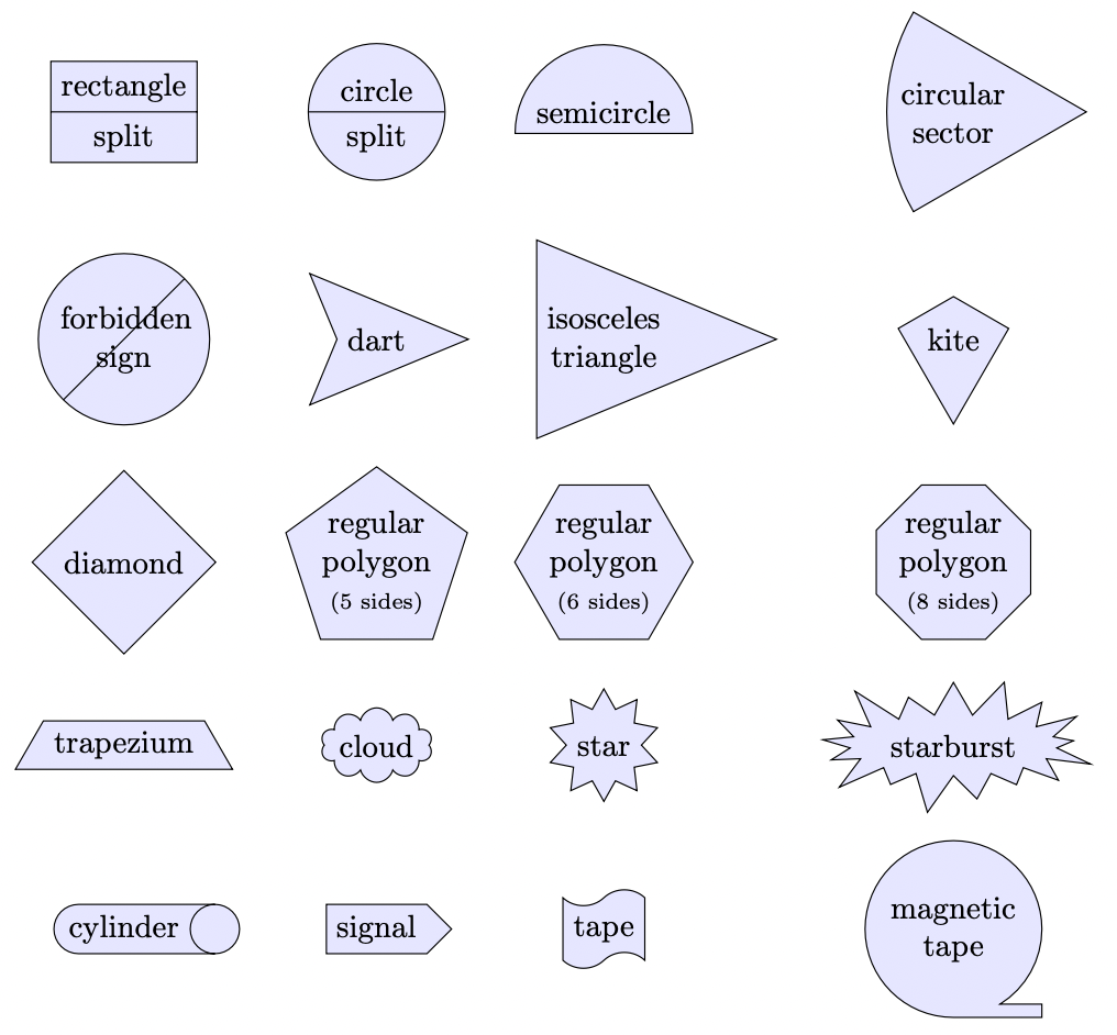
Figure 3.8 – Various node shapes
\documentclass[tikz,border=1pt]{standalone}
\usepackage{tikz}
\usetikzlibrary{shapes,snakes}
\begin{document}
\begin{tikzpicture}
    \matrix[nodes={draw, fill=blue!15},
        row sep=0.2cm, column sep=0.3cm,
        nodes={font=\sffamily}] {
    \node[rectangle split, rectangle split parts=2] {rectangle \nodepart{two} split};&
    \node[circle split] {circle \nodepart{lower} split}; &
    \node[semicircle] {semicircle};&
    \node[circular sector, align=center] {circular\\sector};&
    \\
    \node[forbidden sign,text width=4em, text centered]
                    {forbidden sign};&
    \node[dart] {dart};&
    \node[kite] {kite};&
    \node[isosceles triangle, align=center] {isosceles\\triangle};&
                    \\
    \node[diamond] {diamond};&
    \node[regular polygon, regular polygon sides=5, align=center]
      {regular\\polygon\\(5 sides)};&
    \node[regular polygon, regular polygon sides=6, align=center]
      {regular\\polygon\\(6 sides)};&
    \node[regular polygon, regular polygon sides=8, align=center]
      {regular\\polygon\\(8 sides)};\\
    \node[trapezium] {trapezium};&
    \node[cloud] {cloud};&
    \node[star] {star};&
    \node[starburst] {starburst};&
    \\
    \node[cylinder] {cylinder};&
    \node[signal] {signal};&
    \node[tape] {tape};&
    \node[magnetic tape, align=center] {magnetic\\tape};&
    \\
    };
\end{tikzpicture}
\end{document}

Figure 3.9 – Positioning node shapes
\documentclass[tikz,border=10pt]{standalone}
\usepackage{tikzpeople}
\usetikzlibrary{shapes}
\begin{document}
\begin{tikzpicture}
  \node (student) [graduate, monitor, minimum size=2cm] {};
  \node at (student.45) [starburst, draw=red, fill=yellow,
    starburst point height=0.4cm, line width=1pt,
    font=\ttfamily\scriptsize, inner sep=1.5pt] {error};
  \node at (student.130) [cloud callout, cloud puffs=13, aspect=3,
    anchor=pointer, shading=ball, ball color=darkgray,
    text=white, font=\bfseries] {My thesis...!};
\end{tikzpicture}
\end{document}
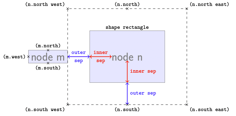
Figure 3.10 – Spacing within and around a node
\documentclass[tikz,border=10pt]{standalone}
\usetikzlibrary{calc}
\begin{document}
\begin{tikzpicture}[font={\scriptsize\ttfamily}]
  \node[draw,rectangle,outer sep=1cm,inner sep=1cm,color=black!50, draw, fill=blue!10]
  (n) {{\sffamily\Large node n}};
  \draw[<->,thick,blue] (n.south)
      --++(0,1cm) node[midway,right]{outer sep};
  \draw[<->,thick,red] (n.south) ++(0,1cm)
      --++(0,1cm)node[midway,right]{inner sep};
  \node[,outer sep=0,draw,left,color=black!50, draw, fill=blue!10,]
      (m) at(n.west) {{\sffamily\Large node m}};
  \draw[<->,blue,thick] (m.east) -- ++(1cm,0) node[midway,above] {outer}
    node[midway,below] {sep};
  \draw[<->,red,thick] ($(n.west)+(1,0)$) -- ++(1cm,0) node[midway,above] {inner}
    node[midway,below] {sep};
  \foreach \anchor/\placement in
    {south west/below left,south/below,north/above,north west/above left,
       north east/above right,south east/below right}
       \draw[shift=(n.\anchor)] plot[mark=x] coordinates{(0,0)}
        node[\placement,label distance = 0mm,inner sep=3pt] {(n.\anchor)};
  \foreach \anchor/\placement in
    {west/left,south/below,north/above}
       \draw[shift=(m.\anchor)] plot[mark=x] coordinates{(0,0)}
        node[\placement,label distance = 0mm,inner sep=3pt] {(m.\anchor)};
  \draw[dashed] (n.south west) rectangle (n.north east);
  \node[above] at ($(n.center)!0.5!(n.north)$) {shape rectangle};
\end{tikzpicture}
\end{document}
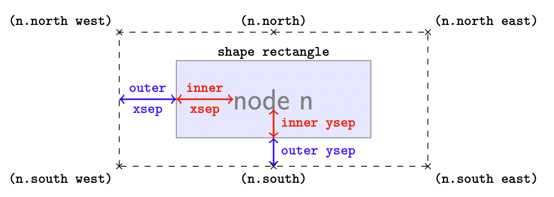
Figure 3.11 – Different horizontal and vertical spacing
\documentclass[tikz,border=10pt]{standalone}
\usetikzlibrary{calc}
\begin{document}
\begin{tikzpicture}[font={\scriptsize\ttfamily}]
  \node[draw,rectangle,outer xsep=1cm,outer ysep=0.5cm,inner xsep=1cm,
    inner ysep=0.5cm,color=black!50, draw, fill=blue!10,] (n) {{\sffamily\Large node n}};
  \draw[<->,thick,blue] (n.south)
      --++(0,0.5cm) node[midway,right]{outer ysep};
  \draw[<->,thick,red] (n.south) ++(0,0.5cm)
      --++(0,0.5cm)node[midway,right]{inner ysep};
  \draw[<->,blue,thick] (n.west) -- ++(1cm,0) node[midway,above] {outer}
    node[midway,below] {xsep};
  \draw[<->,red,thick] ($(n.west)+(1,0)$) -- ++(1cm,0) node[midway,above] {inner}
    node[midway,below] {xsep};
  \foreach \anchor/\placement in
    {south west/below left,south/below,north/above,north west/above left,
       north east/above right,south east/below right}
       \draw[shift=(n.\anchor)] plot[mark=x] coordinates{(0,0)}
        node[\placement,label distance = 0mm,inner sep=3pt] {(n.\anchor)};
  \draw[dashed] (n.south west) rectangle (n.north east);
  \node[above] at ($(n.center)!0.5!(n.north)$) {shape rectangle};
\end{tikzpicture}
\end{document}
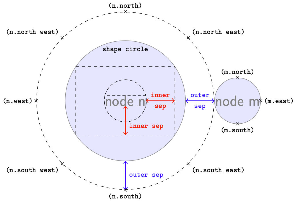
Figure 3.12 – Spacing within and around a circle node
\documentclass[tikz,border=10pt]{standalone}
\usetikzlibrary{calc}
\newcommand{\n}{\sffamily\Large node n}
\newcommand{\invis}{\phantom{\sffamily\Large node n}}
\begin{document}
\begin{tikzpicture}[font={\scriptsize\ttfamily}]
  % node n
  \node[draw,circle,outer sep=1cm,inner sep=1cm,color=black!50, draw, fill=blue!10] (n) {{\n}};
  % label "shape circle"
  \node[above] at ($(n.center)!0.5!(n.north)$) {shape circle};

  % dashed helper nodes with same position and (invisible) same text
  \node[circle,draw,densely dashed,inner sep=0pt,outer sep=0pt] at (n.center) {\invis};
  \node[rectangle,draw,densely dashed,inner sep=0pt,outer sep=0pt] at (n.center) {\invis};
  \node (o) [rectangle,draw, dashed,inner sep=1cm,outer sep=0pt] at (n.center) {\invis};

  % neighbor node
  \node[circle,inner sep=0,outer sep=0,draw,right,color=black!50, draw, fill=blue!10]
      (m) at(n.east) {{\sffamily\Large node m}};

  % vertical sep
  \draw[<->,thick,blue] (n.south)
    --++(0,1cm) node[midway,right]{outer sep};
  \draw[<->,thick,red] (o.south)
    -- ++(0,1cm) node[pos=0.3,right]{inner sep};

  % horizontal sep
  \draw[<->,red,thick] (o.east) -- ++(-1cm,0)
    node[midway,above] {inner} node[midway,below] {sep};
  \draw[<->,blue,thick] (m.west) -- ++(-1cm,0)
    node[midway,above] {outer} node[midway,below] {sep};

% some anchors
  \foreach \anchor/\placement in
    {south west/below left,south/below,north/above,north west/above left,
       north east/above right,south east/below right,west/left}
       \draw[shift=(n.\anchor)] plot[mark=x] coordinates{(0,0)}
        node[\placement,label distance = 0mm,inner sep=3pt] {(n.\anchor)};
  \foreach \anchor/\placement in
    {east/right,south/below,north/above}
       \draw[shift=(m.\anchor)] plot[mark=x] coordinates{(0,0)}
        node[\placement,label distance = 0mm,inner sep=3pt] {(m.\anchor)};

% random circle :-)
\draw[dashed] (n.center) circle (3.05cm);
\end{tikzpicture}
\end{document}

Figure 3.13 – A node above a circle
\documentclass[tikz,border=10pt]{standalone}
\begin{document}
\begin{tikzpicture}
  \draw circle [fill, radius=2pt] node [anchor=south] {text};
\end{tikzpicture}
\end{document}
Different code, same output:
\documentclass[tikz,border=10pt]{standalone}
\begin{document}
\begin{tikzpicture}
  \draw circle [fill, radius=2pt] node [above] {text};
\end{tikzpicture}
\end{document}

Figure 3.14 – A node to the right of another node
\documentclass[tikz,border=10pt]{standalone}
\usetikzlibrary{positioning}
\begin{document}
\begin{tikzpicture}
  \node [draw] (TikZ) {TikZ};
  \node [draw, right = 0.1cm of TikZ] {PDF};
\end{tikzpicture}
\end{document}

Figure 3.15 – A node above and to the right of another node
\documentclass[tikz,border=10pt]{standalone}
\usetikzlibrary{positioning}
\begin{document}
\begin{tikzpicture}
  \node [draw] (TikZ) {TikZ};
  \node [draw, above right = -0.25cm and 0.1cm of TikZ] {PDF};
\end{tikzpicture}
\end{document}
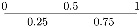
Figure 3.16 – Nodes along a line
\documentclass[tikz,border=10pt]{standalone}
\begin{document}
\begin{tikzpicture}
  \draw (0,0) --
    node [above, pos=0] {0}
    node [above, pos=0.5] {0.5}
    node [above, pos=1] {1}
    node [below, pos=0.25] {0.25}
    node [below, pos=0.75] {0.75}
  (4,0);
\end{tikzpicture}
\end{document}

Figure 3.17 – An epic misalignment
\documentclass[tikz,border=10pt]{standalone}
\usetikzlibrary{positioning}
\begin{document}
\begin{tikzpicture}[every node/.style = {inner sep=0pt}]
  \node (E) {E};
  \node (p) [right = 0pt of E] {p};
  \node (i) [right = 0pt of p] {i};
  \node (c) [right = 0pt of i] {c};
  \node (.) [right = 0pt of c] {.};
\end{tikzpicture}
\end{document}

Figure 3.18 – Epic base alignment
\documentclass[tikz,border=10pt]{standalone}
\usetikzlibrary{positioning}
\begin{document}
\begin{tikzpicture}[every node/.style = {inner sep=0pt}]
  \node (E) {E};
  \node (p) [base right = 0pt of E] {p};
  \node (i) [base right = 0pt of p] {i};
  \node (c) [base right = 0pt of i] {c};
  \node (.) [base right = 0pt of c] {.};
\end{tikzpicture}
\end{document}

Figure 3.19 – Default picture alignment
\documentclass{article}
\usepackage{tikz}
\begin{document}
  \begin{tikzpicture}
    \node[circle, draw, inner sep=2pt] (label) {1};
  \end{tikzpicture}
  This is the first topic.
\end{document}

Figure 3.20 – TikZ picture baseline alignment
\documentclass{article}
\usepackage{tikz}
\begin{document}
  \begin{tikzpicture}[baseline=(label.base)]
    \node[circle, draw, inner sep=2pt] (label) {1};
  \end{tikzpicture}
  This is the first topic.
\end{document}
With a macro, same output:
\documentclass{article}
\usepackage{tikz}
\DeclareRobustCommand{\circled}[1]{\tikz[baseline=(label.base)]{
  \node[circle, draw, inner sep=2pt] (label) {#1};}}
\begin{document}
  \circled{1} This is the first topic.
\end{document}
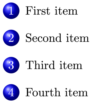
Figure 3.21 – An enumerate environment with fancy TikZ numbers
\documentclass{article}
\usepackage{tikz}
\DeclareRobustCommand{\circled}[1]{%
  \tikz[baseline=(label.base)]{\node[circle,
    white, shading=ball, inner sep=2pt] (label) {#1};}}
\usepackage{enumitem}
\begin{document}
\begin{enumerate}[label=\circled{\arabic*}]
\item First item
\item Second item
\item Third item
\item Fourth item
\end{enumerate}
\end{document}

Figure 3.22 – A node with labels
\documentclass[tikz,border=10pt]{standalone}
\begin{document}
\begin{tikzpicture}[every label/.style = {scale=0.5}]
  \node[
    label = above:Graphics,
    label = left:Design,
    label = below:Typography,
    label = right:Coding,
    circle, shading=ball, ball color=blue!60,
      text=white] {TikZ};
\end{tikzpicture}
\end{document}

Figure 3.23 – A node with pinned labels
\documentclass[tikz,border=10pt]{standalone}
\begin{document}
\begin{tikzpicture}[every pin/.style = {scale=0.5}]
  \node[
    pin = above:Graphics,
    pin = left:Design,
    pin = below:Typography,
    pin = right:Coding,
    circle, shading=ball, ball color=blue!60,
      text=white] {TikZ};
\end{tikzpicture}
\end{document}
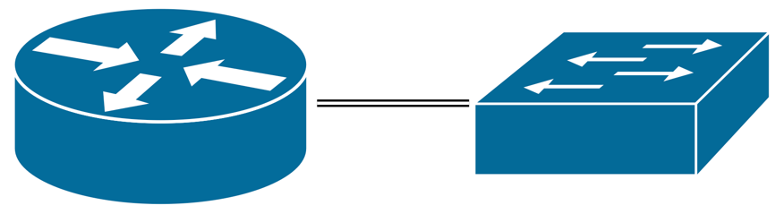
Figure 3.24 – Images in nodes
\documentclass[tikz,border=10pt]{standalone}
\usetikzlibrary{positioning}
\begin{document}
\begin{tikzpicture}
  \node (router) [inner sep=0pt]
    {\includegraphics[width=2cm]{router.pdf}};
  \node (switch) [inner sep=0pt, right = of router]
    {\includegraphics[width=2cm]{switch.pdf}};
  \draw[double] (router) -- (switch);
\end{tikzpicture}
\end{document}
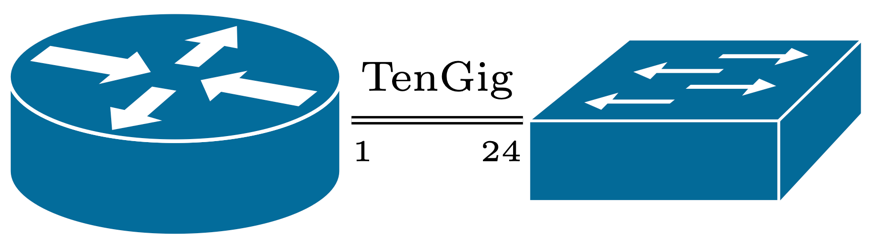
Figure 3.25 – Images in nodes with connection and labels
\documentclass[tikz,border=10pt]{standalone}
\usetikzlibrary{positioning}
\begin{document}
\begin{tikzpicture}
  \node (router) [inner sep=0pt]
    {\includegraphics[width=2cm]{router.pdf}};
  \node (switch) [inner sep=0pt, right = of router]
    {\includegraphics[width=2cm]{switch.pdf}};
  \draw[double] (router) --
    node [above, font=\scriptsize] {TenGig}
    node [font=\tiny, inner xsep=0pt,
      below right, at start] {1}
    node [font=\tiny,inner xsep=0pt,
      below left, at end] {24}
  (switch);
\end{tikzpicture}
\end{document}
Please rate (and possibly review) the book on Amazon if you got it there, your feedback means much to me and helps to get an extended second edition!
Go to next chapter.