Here are the Code examples of this chapter. These pages are currently being updated over time (adding pictures, captions, and possibly further examples). Visit again soon for updates. Of course, the best way to use this page is together with the book for getting the explanations.

Figure 6.1 – A simple tree
\documentclass[tikz,border=10pt]{standalone}
\begin{document}
\begin{tikzpicture}
  \node {A} child { node {1} edge from parent };
\end{tikzpicture}
\end{document}

Figure 6.2 – A customized edge in a tree
\documentclass[tikz,border=10pt]{standalone}
\begin{document}
\begin{tikzpicture}
  \node {A} child { node {1}
    edge from parent [dashed, ->]
    node[above, sloped, font=\tiny] {down} };
\end{tikzpicture}
\end{document}
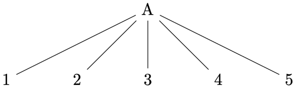
Figure 6.3 – A tree with five children
\documentclass[tikz,border=10pt]{standalone}
\begin{document}
\begin{tikzpicture}
  \node {A}
    child { node {1} }
    child { node {2} }
    child { node {3} }
    child { node {4} }
    child { node {5} }
  ;
\end{tikzpicture}
\end{document}
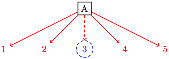
Figure 6.4 – A tree with custom style options
\documentclass[tikz,border=10pt]{standalone}
\begin{document}
\begin{tikzpicture}[thick]
  \node [draw, black, rectangle] {A}
    [red, ->]
    child { node {1} }
    child { node {2} }
    child [densely dashed]
      { node [draw, blue, circle] {3} }
    child { node {4} }
    child { node {5} }
  ;
\end{tikzpicture}
\end{document}
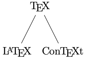
Figure 6.5 – A minimal TeX relationship tree
\documentclass[tikz,border=10pt]{standalone}
\usepackage{hvlogos}
\begin{document}
\begin{tikzpicture}
  \node {\TeX}
    child { node {\LaTeX} }
    child { node {\ConTeXt} }
  ;
\end{tikzpicture}
\end{document}
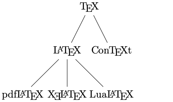
Figure 6.6 – A TeX and LaTeX relationship tree
\documentclass[tikz,border=10pt]{standalone}
\usepackage{hvlogos}
\begin{document}
\begin{tikzpicture}
  \node {\TeX}
    child { node {\LaTeX}
      child { node {\pdfLaTeX} }
      child { node {\XeLaTeX} }
      child { node {\LuaLaTeX} }
    }
    child { node {\ConTeXt} }
  ;
\end{tikzpicture}
\end{document}
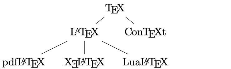
Figure 6.7 – Adjusted distances in a tree
\documentclass[tikz,border=10pt]{standalone}
\usepackage{hvlogos}
\begin{document}
\begin{tikzpicture}[
  level 1/.style = { level distance   = 8mm,
                     sibling distance = 20mm },
  level 2/.style = { level distance   = 10mm,
                     sibling distance = 20mm } ]
  \node {\TeX}
    child { node {\LaTeX}
      child { node {\pdfLaTeX} }
      child { node {\XeLaTeX} }
      child { node {\LuaLaTeX} }
    }
    child { node {\ConTeXt} }
  ;
\end{tikzpicture}
\end{document}
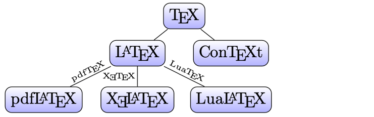
Figure 6.8 – A colored tree
\documentclass[tikz,border=10pt]{standalone}
\usepackage{hvlogos}
\begin{document}
\begin{tikzpicture}[
  level 1/.style = { level distance = 8mm,
                     sibling distance = 20mm },
  level 2/.style = { level distance = 10mm,
                     sibling distance = 20mm },
  treenode/.style = {shape = rectangle,
    rounded corners, draw,
    top color=white, bottom color=blue!30},
  every child node/.style = {treenode},
  engine/.style = {inner sep = 1pt, font=\tiny, above}
]
\node [treenode] {\TeX}
  child { node {\LaTeX}
    child { node {\pdfLaTeX}
      edge from parent node[engine, sloped] {\pdfTeX}}
    child { node {\XeLaTeX}
      edge from parent node[engine, left]   {\XeTeX} }
    child { node {\LuaLaTeX}
      edge from parent node[engine, sloped] {\LuaTeX}}
  }
  child { node {\ConTeXt} }
;
\end{tikzpicture}
\end{document}
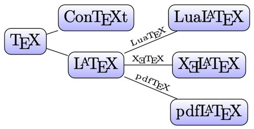
Figure 6.9 – A tree from left to right
\documentclass[tikz,border=10pt]{standalone}
\usepackage{hvlogos}
\begin{document}
\begin{tikzpicture}[
  level 1/.style = { level distance = 16mm,
                     sibling distance = 10mm },
  level 2/.style = { level distance = 30mm,
                     sibling distance = 10mm },
  treenode/.style = {shape = rectangle,
    rounded corners, draw,
    top color=white, bottom color=blue!30},
  every child node/.style = {treenode},
  engine/.style = {inner sep=1pt, font = \tiny, sloped, above},
  grow = right
]
\node [treenode] {\TeX}
  child { node {\LaTeX}
    child { node {\pdfLaTeX} edge from parent node[engine] {\pdfTeX}}
    child { node {\XeLaTeX} edge from parent node[engine] {\XeTeX} }
    child { node {\LuaLaTeX} edge from parent node[engine] {\LuaTeX}}
  }
  child { node {\ConTeXt} }
;
\end{tikzpicture}
\end{document}
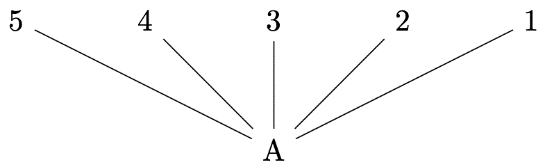
Figure 6.10 – A tree growing up
\documentclass[tikz,border=10pt]{standalone}
\begin{document}
\begin{tikzpicture}[grow=up]
\node {A}
  child { node {1} }
  child { node {2} }
  child { node {3} }
  child { node {4} }
  child { node {5} }
;
\end{tikzpicture}
\end{document}
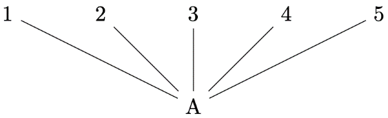
Figure 6.11 – A tree growing up with children in inverted order
\documentclass[tikz,border=10pt]{standalone}
\begin{document}
\begin{tikzpicture}[grow'=up]
\node {A}
  child { node {1} }
  child { node {2} }
  child { node {3} }
  child { node {4} }
  child { node {5} }
;
\end{tikzpicture}
\end{document}
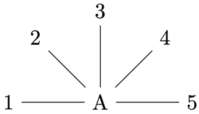
Figure 6.12 – A tree with a circular child node arrangement
\documentclass[tikz,border=10pt]{standalone}
\usetikzlibrary{trees}
\begin{document}
\begin{tikzpicture}[clockwise from = 180,
  sibling angle=45]
\node {A} child { node {1} };
\node {A}
  child { node {1} }
  child { node {2} }
  child { node {3} }
  child { node {4} }
  child { node {5} }
;
\end{tikzpicture}
\end{document}

Figure 6.13 – A minimal mind map
\documentclass[tikz,border=10pt]{standalone}
\usetikzlibrary{mindmap}
\begin{document}
\begin{tikzpicture}[
    mindmap,
    concept color = blue!50,
    text = white,
  ]
  \node [concept, font=\Huge\sffamily\bfseries] {TikZ}
    child [clockwise from = 0] {
      node [concept, font=\Large\sffamily] {Graphs}
  };
\end{tikzpicture}
\end{document}
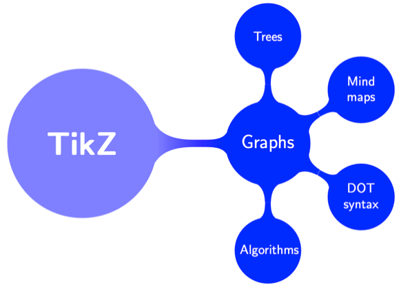
Figure 6.14 – A mind map with root and two levels
\documentclass[tikz,border=10pt]{standalone}
\usetikzlibrary{mindmap}
\begin{document}
\begin{tikzpicture}[
  mindmap,
  text = white,
  concept color = blue!50,
  nodes = {concept},
  root/.append style = {
    font = \Huge\sffamily\bfseries},
  level 1 concept/.append style =
    {font = \Large\sffamily, sibling angle=90},
  level 2 concept/.append style =
    {font = \normalsize\sffamily}
  ]
  \node [root] {TikZ} [clockwise from=0]
    child [concept color=blue] {
      node {Graphs} [clockwise from=90]
        child { node {Trees} }
        child { node {Mind maps} }
        child { node {DOT syntax} }
        child { node {Algorithms} }
    };
\end{tikzpicture}
\end{document}
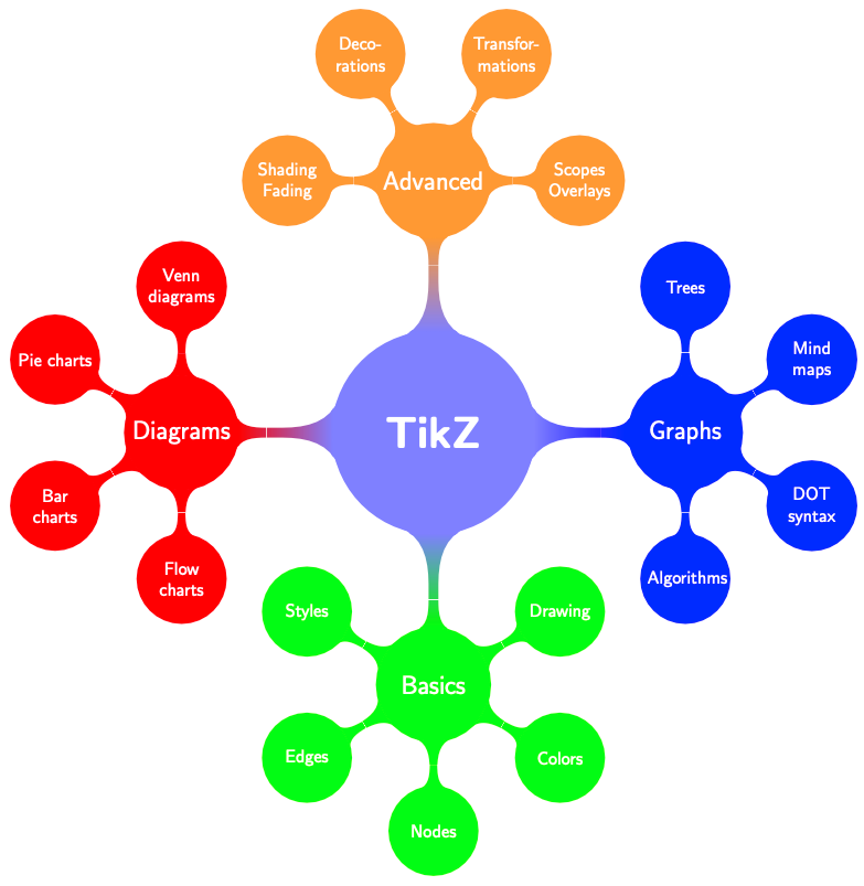
Figure 6.15 – A comprehensive mind map
\documentclass[tikz,border=10pt]{standalone}
\usetikzlibrary{mindmap}
\begin{document}
\begin{tikzpicture}[
  mindmap,
  text = white,
  concept color = blue!50,
  nodes = {concept},
  root/.append style = {
    font = \Huge\sffamily\bfseries},
  level 1 concept/.append style =
    {font = \Large\sffamily, sibling angle=90},
  level 2 concept/.append style =
    {font = \normalsize\sffamily}
  ]
  \node [root] {TikZ} [clockwise from=0]
    child [concept color=blue] {
      node {Graphs} [clockwise from=90]
        child { node {Trees} }
        child { node {Mind maps} }
        child { node {DOT syntax} }
        child { node {Algorithms} }
    }
    child [concept color=green] {
      node {Basics} [clockwise from=30]
        child { node {Drawing} }
        child { node {Colors} }
        child { node {Nodes} }
        child { node {Edges} }
        child { node {Styles} }
    }
    child [concept color=red] {
      node {Diagrams} [clockwise from=-90]
        child { node {Flow charts} }
        child { node {Bar charts} }
        child { node {Pie charts} }
        child { node {Venn diagrams} }
    }
    child [concept color=orange!80] {
      node {Advanced} [clockwise from=180]
        child { node {Shading\\Fading} }
        child { node {Deco\-rations} }
        child { node {Transfor\-mations} }
        child { node {Scopes\\Overlays} }
    };
\end{tikzpicture}
\end{document}
Producing graphs

Figure 6.16 – A simple graph
\documentclass[tikz,border = 10pt]{standalone}
\usetikzlibrary{graphs}
\begin{document}
\begin{tikzpicture}[nodes = {text depth = 1ex,
    text height = 2ex}]
  \graph { tex -> dvi -> ps -> pdf };
\end{tikzpicture}
\end{document}
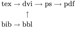
Figure 6.17 – Node chains in a graph
\documentclass[tikz,border = 10pt]{standalone}
\usetikzlibrary{graphs}
\begin{document}
\begin{tikzpicture}[nodes = {text depth = 1ex,
    text height = 2ex}]
  \graph { tex -> dvi -> ps -> pdf,
           bib -> bbl,
           bbl -> dvi };
\end{tikzpicture}
\end{document}
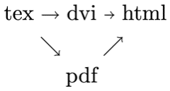
Figure 6.18 – Node groups
\documentclass[tikz,border = 10pt]{standalone}
\usetikzlibrary{graphs}
\begin{document}
\begin{tikzpicture}[nodes = {text depth = 1ex,
    text height = 2ex}]
  \graph { tex -> {dvi, pdf } -> html };
\end{tikzpicture}
\end{document}

Figure 6.19 – Node distance in a graph
\documentclass[tikz,border = 10pt]{standalone}
\usetikzlibrary{graphs}
\begin{document}
\begin{tikzpicture}[nodes = {text depth = 1ex,
    text height = 2ex}]
  \graph [grow right = 2cm] { tex -> dvi -> ps -> pdf };
\end{tikzpicture}
\end{document}

Figure 6.20 – Edge quotes in a graph
\documentclass[tikz,border = 10pt]{standalone}
\usetikzlibrary{graphs,quotes}
\begin{document}
\begin{tikzpicture}[nodes = {text depth = 1ex,
    text height = 2ex},
    every edge quotes/.style = {font=\tiny\ttfamily,
  above, inner sep = 0pt}]
  \graph [grow right = 2cm]
    { tex -> ["latex"] dvi
          -> ["dvips"] ps -> ["ps2pdf"] pdf };
\end{tikzpicture}
\end{document}
Positioning in a matrix

Figure 6.21 – A simple matrix node
\documentclass[tikz,border = 10pt]{standalone}
\begin{document}
\begin{tikzpicture}
  \node[matrix,draw]  {
    \node{A}; & \node{B}; & \node{C}; \\
    \node{D}; & \node{E}; & \node{F}; \\
  };
\end{tikzpicture}
\end{document}
With the matrix library
\documentclass[tikz,border = 10pt]{standalone}
\usetikzlibrary{matrix}
\begin{document}
\begin{tikzpicture}
  \matrix[matrix of nodes, draw] {
    A & B & C \\
    D & E & F \\
  };
\end{tikzpicture}
\end{document}
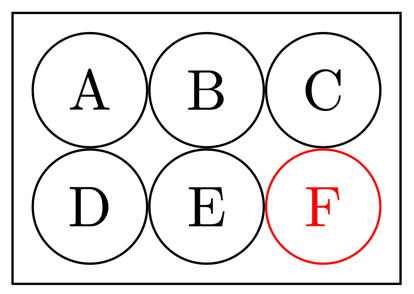
Figure 6.22 – Matrix cell nodes with style options
\documentclass[tikz,border = 10pt]{standalone}
\usetikzlibrary{matrix}
\begin{document}
\begin{tikzpicture}
  \matrix [matrix of nodes, draw,
      nodes = {circle, draw, minimum width=2em} ] {
    A & B & C \\
    D & E & |[red]|F \\
   };
\end{tikzpicture}
\end{document}
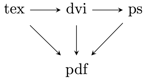
Figure 6.23 – A matrix diagram with arrows
\documentclass[tikz,border = 10pt]{standalone}
\usetikzlibrary{matrix}
\begin{document}
\begin{tikzpicture}
  \matrix (m) [matrix of nodes,
    row sep = 2em, column sep = 2em,
    nodes = {text depth = 1ex, text height = 2ex}
  ]
  {
    tex & dvi & ps \\
        & pdf &    \\
  };
  \draw [-stealth]
    (m-1-1) edge (m-1-2)
    (m-1-2) edge (m-1-3)
    (m-1-1) edge (m-2-2)
    (m-1-2) edge (m-2-2)
    (m-1-3) edge (m-2-2)
  ;
\end{tikzpicture}
\end{document}
Named matrix nodes
\documentclass[tikz,border = 10pt]{standalone}
\usetikzlibrary{matrix}
\begin{document}
\begin{tikzpicture}
  \matrix (m) [matrix of nodes,
    row sep = 2em, column sep = 2em,
    nodes = {text depth = 1ex, text height = 2ex}
  ]
  {
    tex & |(d)|dvi & ps \\
        & |(p)|pdf &    \\
  };
  \draw (d) -- (p);
\end{tikzpicture}
\end{document}
Please rate (and possibly review) the book on Amazon if you got it there, your feedback means much to me and helps to get an extended second edition!
Go to next chapter.