Here are the Code examples of this chapter. These pages are currently being updated over time (adding pictures, captions, and possibly further examples). Visit again soon for updates. Of course, the best way to use this page is together with the book for getting the explanations.
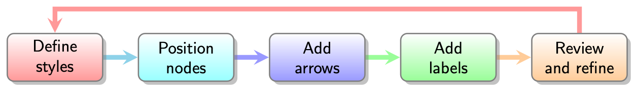
Figure 14.1 – A flowchart depicting a diagram creation process
\documentclass[tikz,border=10pt]{standalone}
\usepackage{smartdiagram}
\smartdiagramset{font=\sffamily}
\begin{document}
\smartdiagram[flow diagram:horizontal]{
  Define Styles, Position nodes, Add arrows,
  Add labels, Review and refine}
\end{document}
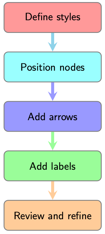
Figure 14.2 – A vertical flowchart with flat colors and without shadows
\documentclass[tikz,border=10pt]{standalone}
\usepackage{smartdiagram}
\smartdiagramset{font=\sffamily,
   text width = 3cm, back arrow disabled}
\tikzset{module/.append style=
  { top color=\col, bottom color=\col},
  every shadow/.style = {fill=none, shadow scale=0}}
\begin{document}
\smartdiagram[flow diagram]{
  Define styles, Position nodes, Add arrows,
  Add labels, Review and refine}
\end{document}

Figure 14.3 – A sequence diagram with custom colors
\documentclass[tikz,border=10pt]{standalone}
\usepackage{smartdiagram}
\begin{document}
\smartdiagramset{sequence item font size=\sffamily\Large\strut,
   set color list={red!80, red!60, red!45, red!30} }
\tikzset{module/.append style = {top color=\col} }
\smartdiagram[sequence diagram]{
  Styles, Positions, Arrows, Labels}
\end{document}
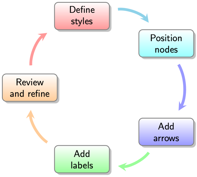
Figure 14.4 – A circular diagram
\documentclass[tikz,border=10pt]{standalone}
\usepackage{smartdiagram}
\smartdiagramset{font=\sffamily}
\begin{document}
\smartdiagram[circular diagram:clockwise]{
  Define styles, Position nodes, Add arrows,
  Add labels, Review and refine}
\end{document}
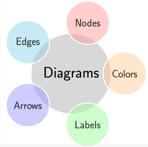
Figure 14.5 – A bubble diagram
\documentclass[tikz,border=10pt]{standalone}
\usepackage{smartdiagram}
\smartdiagramset{bubble node font=\sffamily\Large,
 bubble center node font=\sffamily\Huge}
\begin{document}
\smartdiagram[bubble diagram]{Diagrams,
      Nodes, Edges, Arrows, Labels, Colors}
\end{document}
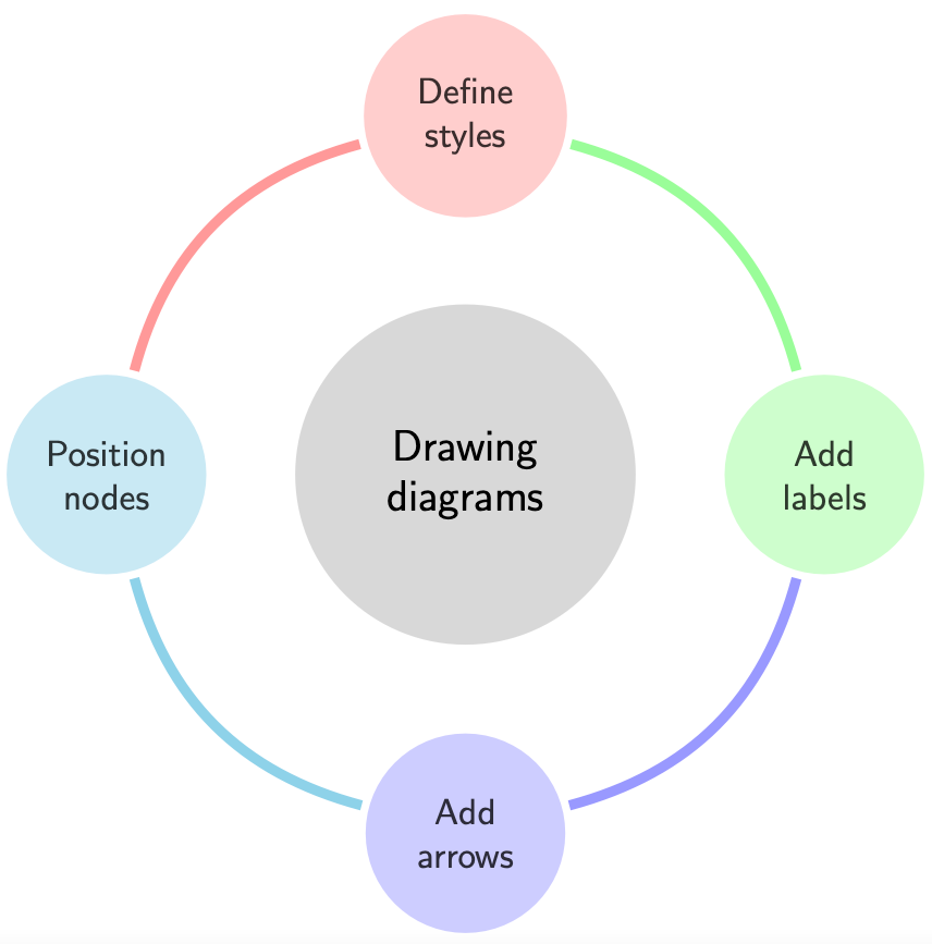
Figure 14.6 – A connected constellation diagram
\documentclass[tikz,border=10pt]{standalone}
\usepackage{smartdiagram}
\smartdiagramset{planet font=\sffamily\LARGE,
  planet text width=2.2cm,
  satellite font=\sffamily}
\begin{document}
\smartdiagram[connected constellation diagram]{
  Drawing diagrams, Define styles,
  Position nodes, Add arrows, Add labels}
\end{document}
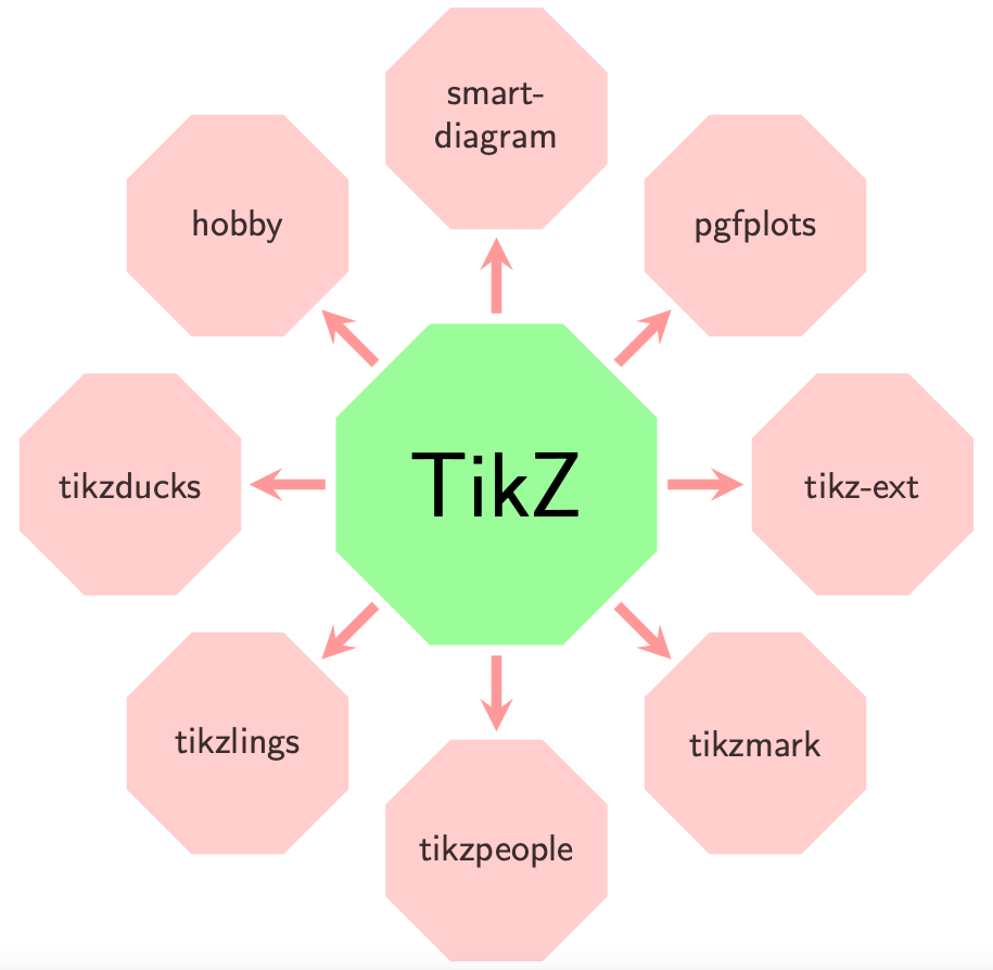
Figure 14.7 – A constellation diagram with arrows
\documentclass[tikz,border=10pt]{standalone}
\usepackage{smartdiagram}
\usetikzlibrary{shapes.geometric}
\smartdiagramset{planet font=\sffamily\Huge,
   satellite font=\sffamily,
   planet color=green!40, uniform connection color=true,
   uniform color list = red!40 for 8 items}
\tikzset{satellite/.append style={regular polygon,
  regular polygon sides=8, inner sep=0pt},
  planet/.append style={regular polygon,
  regular polygon sides=8, inner sep=6pt}}
\begin{document}
\smartdiagram[constellation diagram]{TikZ,
  pgfplots, smartdiagram, hobby, tikzducks,
  tikzlings, tikzpeople, tikzmark, tikz-ext}
\end{document}
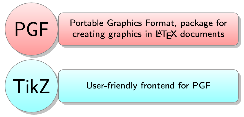
Figure 14.8 – A descriptive diagram
\documentclass[tikz,border=10pt]{standalone}
\usepackage{smartdiagram}
\begin{document}
\smartdiagramset{description title font=\sffamily\LARGE,
  description font=\sffamily\footnotesize}
\smartdiagram[descriptive diagram]{
  {PGF,{Portable Graphics Format, package for
        creating graphics in \LaTeX{} documents}},
  {TikZ, {User-friendly frontend for PGF}},}
\end{document}
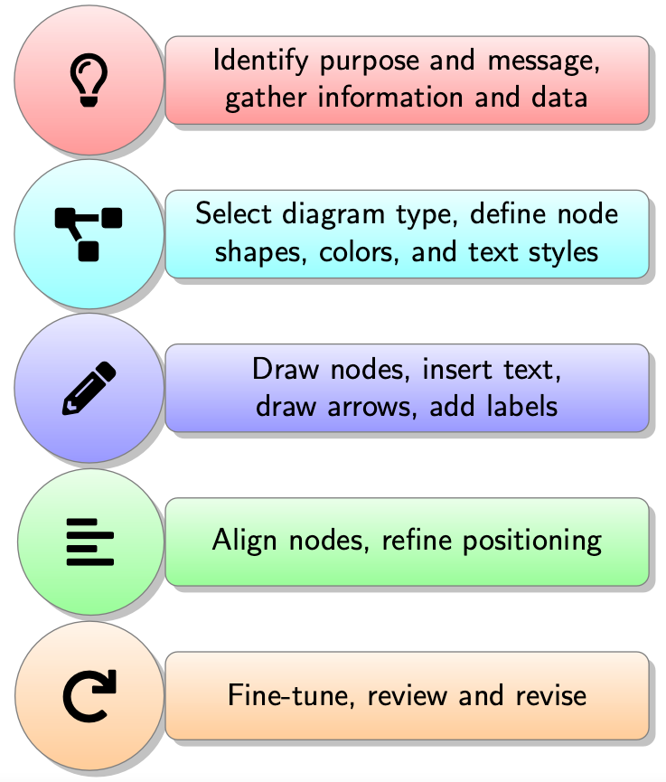
Figure 14.9 – A customized bullet list diagram
\documentclass[tikz,border=10pt]{standalone}
\usepackage{smartdiagram}
\usepackage{fontawesome5}
\begin{document}
\smartdiagramset{description title font=\LARGE,
  description font=\sffamily}
\smartdiagram[descriptive diagram]{
  {\faLightbulb[regular],{Identify purpose and message,
    gather information and data}},
  {\faProjectDiagram, {Select diagram type,
    define node shapes, colors, and text styles}},
  {\faPencil*, {Draw nodes, insert text, draw arrows,
    add labels}},
  {\faAlignLeft, {Align nodes, refine positioning}},
  {\faRedo, {Fine-tune, review and revise}}, }
\end{document}
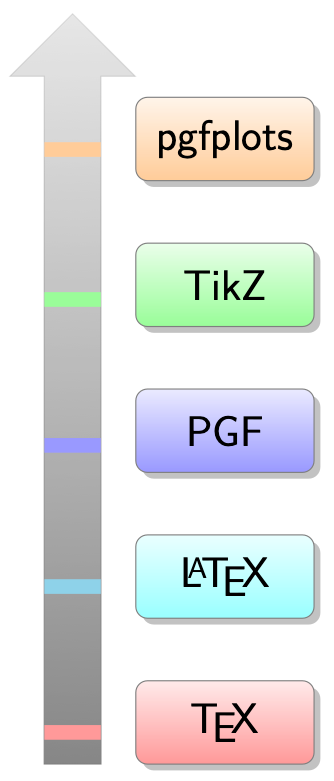
Figure 14.10 – A priority descriptive diagram
\documentclass[tikz,border=10pt]{standalone}
\usepackage{smartdiagram}
\begin{document}
\smartdiagramset{description font=\sffamily\Large,
  description text width = 1.9cm,
  description width = 2cm}
\smartdiagram[priority descriptive diagram]{
      \TeX, \LaTeX, PGF, TikZ, pgfplots}
\end{document}
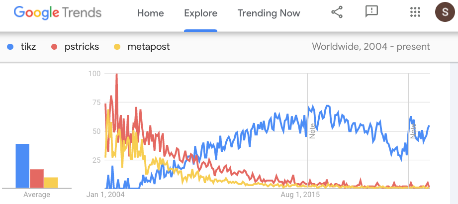
Figure 14.11 – A Google Trends chart for LaTeX graphics packages
Source: Google Trends
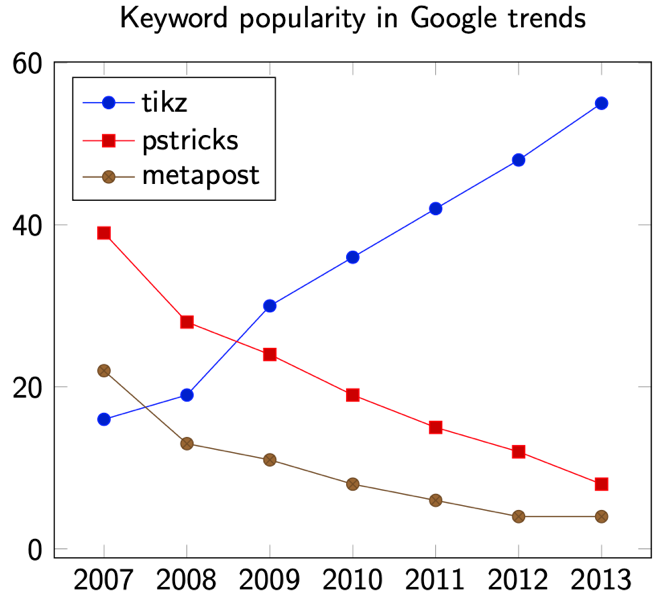
Figure 14.12 – A line chart representing keyword popularity over time
\documentclass[border=10pt]{standalone}
\usepackage{pgfplots}
\tikzset{every node/.style={font=\sffamily}}
\usepackage{sansmath}
\pgfplotsset{tick label style = {font=\sansmath}}
\begin{document}
\begin{tikzpicture}
  \begin{axis}[title  = Keyword popularity in Google trends,
    x tick label style =
      {/pgf/number format/set thousands separator={}},
    legend pos = north west,
    legend cell align=left ]
  \addplot coordinates { (2007,16) (2008,19) (2009,30) (2010,36)
    (2011,42) (2012,48) (2013,55)};
  \addplot coordinates { (2007,39) (2008,28) (2009,24) (2010,19)
    (2011,15) (2012,12) (2013,8)};
  \addplot coordinates { (2007,22) (2008,13) (2009,11) (2010,8)
    (2011,6) (2012,4) (2013,4)};
  \legend{tikz, pstricks, metapost}
  \end{axis}
\end{tikzpicture}
\end{document}
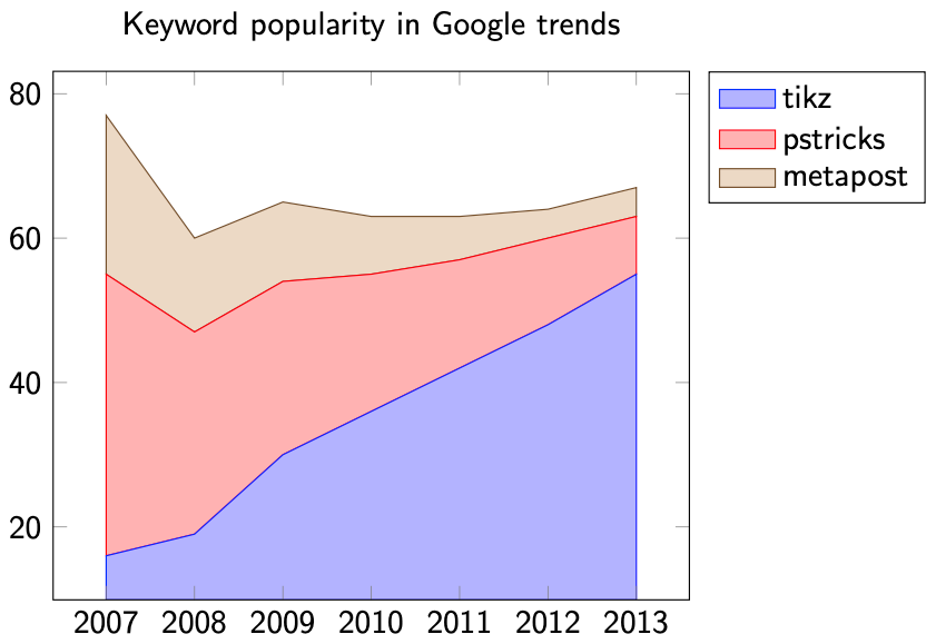
Figure 14.13 – A stacked line chart showing cumulated values and relative proportions
\documentclass[border=10pt]{standalone}
\usepackage{pgfplots}
\usepackage{sansmath}
\pgfplotsset{tick label style = {font=\sansmath\sffamily}}
\begin{document}
\begin{tikzpicture}[every node/.style={font=\sffamily}]
  \begin{axis}[title  = Keyword popularity in Google trends,
    stack plots=y,
    area style,
    x tick label style =
      {/pgf/number format/set thousands separator={}},
    legend pos = outer north east,
    legend cell align=left ]
  \addplot coordinates { (2007,16) (2008,19) (2009,30) (2010,36)
    (2011,42) (2012,48) (2013,55)}\closedcycle;;
  \addplot coordinates { (2007,39) (2008,28) (2009,24) (2010,19)
    (2011,15) (2012,12) (2013,8)}\closedcycle;;
  \addplot coordinates { (2007,22) (2008,13) (2009,11) (2010,8)
    (2011,6) (2012,4) (2013,4)}\closedcycle;;
  \legend{tikz, pstricks, metapost}
  \end{axis}
\end{tikzpicture}
\end{document}
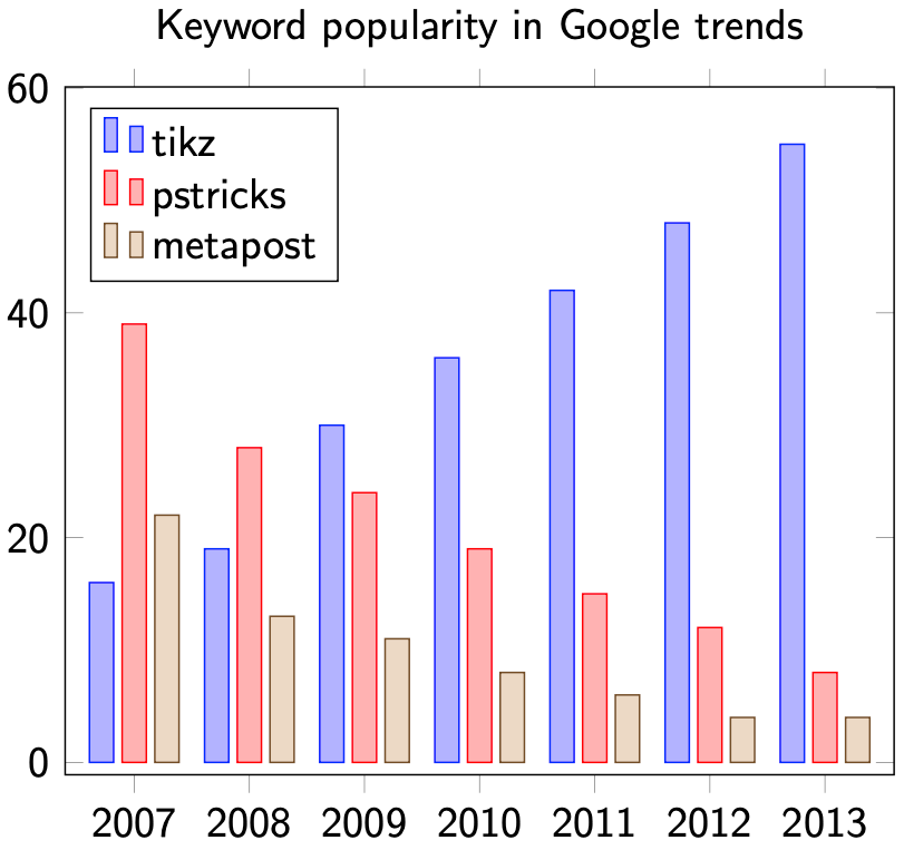
Figure 14.14 – A bar chart visualizing relative and absolute values over time
\documentclass[border=10pt]{standalone}
\usepackage{pgfplots}
\usepackage{sansmath}
\pgfplotsset{tick label style = {font=\sansmath\sffamily}}
\begin{document}
\begin{tikzpicture}[every node/.style={font=\sffamily}]
  \begin{axis}[title  = Keyword popularity in Google trends,
    ybar,
    bar width=2mm,
    x tick label style =
      {/pgf/number format/set thousands separator={}},
  legend pos=north west,
  legend cell align=left]
  \addplot coordinates { (2007,16) (2008,19) (2009,30) (2010,36)
    (2011,42) (2012,48) (2013,55)};
  \addplot coordinates { (2007,39) (2008,28) (2009,24) (2010,19)
    (2011,15) (2012,12) (2013,8)};
  \addplot coordinates { (2007,22) (2008,13) (2009,11) (2010,8)
    (2011,6) (2012,4) (2013,4)};
  \legend{tikz, pstricks, metapost}
  \end{axis}
\end{tikzpicture}
\end{document}
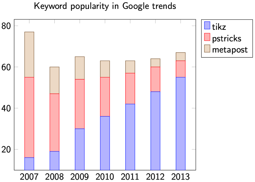
Figure 14.15 – A stacked bar chart showing cumulated values and relative proportions
\documentclass[border=10pt]{standalone}
\usepackage{pgfplots}
\usepackage{sansmath}
\pgfplotsset{tick label style = {font=\sansmath\sffamily}}
\begin{document}
\begin{tikzpicture}[every node/.style={font=\sffamily}]
  \begin{axis}[title  = Keyword popularity in Google trends,
    ybar stacked,
    x tick label style =
      {/pgf/number format/set thousands separator={}},
    legend pos = outer north east,
    legend cell align=left]
  \addplot coordinates { (2007,16) (2008,19) (2009,30) (2010,36)
    (2011,42) (2012,48) (2013,55)};
  \addplot coordinates { (2007,39) (2008,28) (2009,24) (2010,19)
    (2011,15) (2012,12) (2013,8)};
  \addplot coordinates { (2007,22) (2008,13) (2009,11) (2010,8)
    (2011,6) (2012,4) (2013,4)};
  \legend{tikz, pstricks, metapost}
  \end{axis}
\end{tikzpicture}
\end{document}
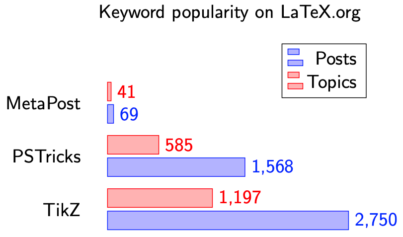
Figure 14.16 – A horizontal bar chart with symbolic coordinates
\documentclass[border=10pt]{standalone}
\usepackage{pgfplots}
\pgfplotsset{compat=1.18}
\usepackage{sansmath}
\begin{document}
\begin{tikzpicture}[every node/.style={font=\sffamily}]
  \begin{axis}[title  = Keyword popularity on LaTeX.org,
    height=6cm, enlarge y limits  = 0.6,
    xbar,
    axis x line = none,
    y axis line style = transparent,
    ytick = data,
    tickwidth = 0pt,
    symbolic y coords = {TikZ, PSTricks, MetaPost},
    nodes near coords,
    nodes near coords style = {font=\sansmath},
    legend cell align = right ]
  \addplot coordinates { (2750,TikZ) (1568,PSTricks)
                         (69,MetaPost) };
  \addplot coordinates { (1197,TikZ) (585,PSTricks)
                         (41,MetaPost)};
  \legend{Posts,Topics}
  \end{axis}
\end{tikzpicture}
\end{document}
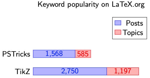
Figure 14.17 – A stacked horizontal bar chart
\documentclass[border=10pt]{standalone}
\usepackage{pgfplots}
\pgfplotsset{compat=1.18}
\usepackage{sansmath}
\begin{document}
\begin{tikzpicture}[every node/.style={font=\sffamily}]
  \begin{axis}[title  = Keyword popularity on LaTeX.org,
    height=6cm, enlarge y limits  = 2.2,
    xbar stacked, xmin=-10,
    axis x line = none,
    y axis line style = transparent,
    ytick = data,
    tickwidth = 0pt,
    symbolic y coords = {TikZ, PSTricks, MetaPost},
    nodes near coords,
    nodes near coords style = {font=\sansmath},
    legend cell align = right ]
    \addplot coordinates { (2750,TikZ) (1568,PSTricks) };
    \addplot coordinates { (1197,TikZ) (585,PSTricks)  };
    \legend{Posts,Topics}
  \end{axis}
\end{tikzpicture}
\end{document}
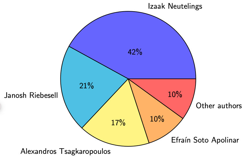
Figure 14.18 – A pie chart
\documentclass[border=10pt]{standalone}
\usepackage{pgf-pie}
\begin{document}
\begin{tikzpicture}[every node/.style={font=\sffamily}]
  \pie{ 42/Izaak Neutelings,
        21/Janosh Riebesell,
        17/Alexandros Tsagkaropoulos,
        10/Efraín Soto Apolinar,
        10/Other authors }
\end{tikzpicture}
\end{document}
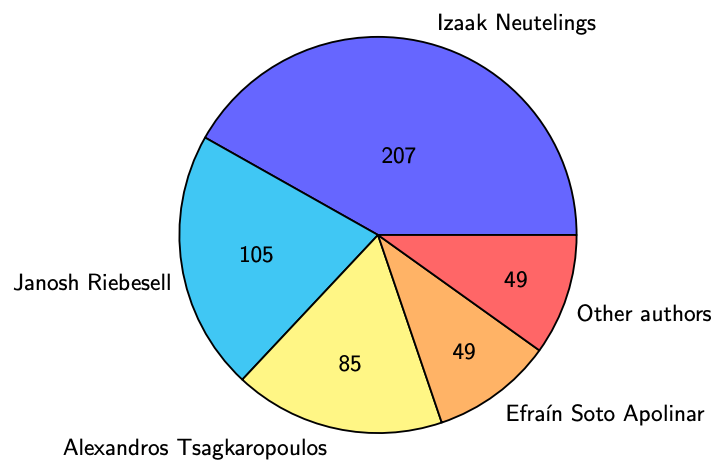
Pie chart with absolute values and auto-summation
\documentclass[border=10pt]{standalone}
\usepackage{pgf-pie}
\begin{document}
\begin{tikzpicture}[every node/.style={font=\sffamily}]
  \pie[sum=auto]{ 207/Izaak Neutelings,
        105/Janosh Riebesell,
        85/Alexandros Tsagkaropoulos,
        49/Efraín Soto Apolinar,
        49/Other authors }
\end{tikzpicture}
\end{document}
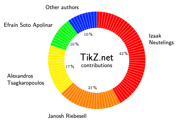
Figure 14.19 – A wheel chart
\documentclass[border=10pt]{standalone}
\usepackage{wheelchart}
\begin{document}
\begin{tikzpicture}[every node/.style={font=\sffamily}]
  \wheelchart [middle={{\LARGE TikZ.net}\\contributions},
    inner data = {\scriptsize\WCperc}, inner data sep=0.3,
    wheel lines=white]
    {42/red/Izaak\\Neutelings,
     21/orange/Janosh Riebesell,
     17/yellow/Alexandros\\Tsagkaropoulos,
     10/green/Efraín Soto Apolinar,
     10/blue/Other authors}
\end{tikzpicture}
\end{document}
Please rate (and possibly review) the book on Amazon if you got it there, your feedback means much to me and helps to get an extended second edition!
Go to next chapter.