Here are the Code examples of this chapter. These pages are currently being updated over time (adding pictures, captions, and possibly further examples). Visit again soon for updates. Of course, the best way to use this page is together with the book for getting the explanations.
Having to re-upload the images these days
Testing simple transformations
\documentclass[tikz,border=10pt]{standalone}
\usetikzlibrary{calc}
\begin{document}
\begin{tikzpicture}
  \draw[thin,dotted] (-1,-1) grid (3,3);
  \draw[->] (-1,0) -- (3.2,0);
  \draw[->] (0,-1) -- (0,3.2);
  \draw[yshift=2cm] (0,0) -- (1,1);
  \draw[xshift=1cm, yshift=2cm] (0,0) circle(1);
  \draw[shift={(1cm,2cm)}] (0,0) circle(1);
  \draw ([shift={(2,3)}]1,1) -- (4,5);
  \draw ($(1,1)+(3,4)$) -- (4,5);
  \coordinate (A) at (-3, 1);
  \coordinate (B) at (-1, 1);
  \draw (A) -- (B) node[pos=0.5, yshift=2mm] {text};
  \draw[yshift=2cm] (A) -- (B);
  \draw ([yshift=2cm]A.east) -- ([yshift=2cm]B.west);
\end{tikzpicture}
\end{document}
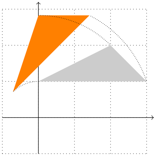
Figure 11.1 – Rotating a triangle around the origin
\documentclass[tikz,border=10pt]{standalone}
\begin{document}
\begin{tikzpicture}
  % grid and coordinate axes:
  \draw[thin,dotted] (-1,-1) grid (3,3);
  \draw[->] (-1,0) -- (3,0);
  \draw[->] (0,-1) -- (0,3);
  % original triangle:
  \fill[gray!40] (0,1) -- (3,1) -- (2,2) --cycle;
  % rotated triangle:
  \fill[orange, rotate=45] (0,1) -- (3,1) -- (2,2) --cycle;
  % clipped circles to show the rotation:
  \begin{scope}
    \clip (0,1) rectangle (3,2.82);
    \draw[densely dotted] circle(3.16);
  \end{scope}
  \begin{scope}
    \clip (0,3) rectangle (2,2);
    \draw[densely dotted] circle(2.83);
  \end{scope}
  \begin{scope}
    \clip (-0.7,0.6) rectangle (0,1);
    \draw[densely dotted] circle(1);
  \end{scope}
\end{tikzpicture}
\end{document}
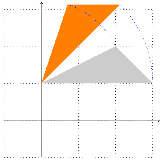
Figure 11.2 – Rotating a triangle around a point
\documentclass[tikz,border=10pt]{standalone}
\begin{document}
\begin{tikzpicture}
  \draw[thin,dotted] (-1,-1) grid (3,3);
  \draw[->] (-1,0) -- (3.2,0);
  \draw[->] (0,-1) -- (0,3.2);
  % original triangle:
  \fill[gray!40] (0,1) -- (3,1) -- (2,2) --cycle;
  % rotated triangle:
  \fill[orange,rotate around={45:(0,1)}]
    (0,1) -- (3,1) -- (2,2) --cycle;
  % clipped circles to show the rotation:
  \begin{scope}
    \clip (2.1,3.1) rectangle (3,1);
    \draw[blue, densely dotted] (0,1) circle(3);
  \end{scope}
  \begin{scope}
    \clip (0.72,3.2) rectangle (2,2);
    \draw[blue, densely dotted] (0,1) circle(2.24);
  \end{scope}
\end{tikzpicture}
\end{document}
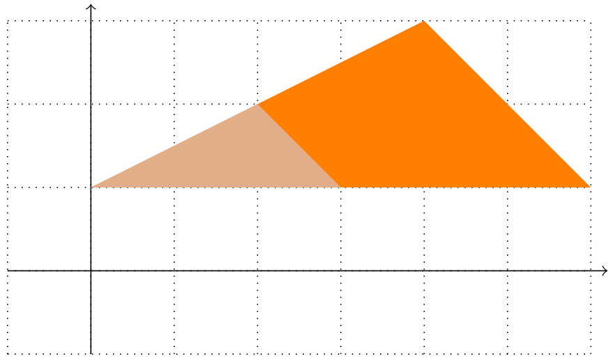
Figure 11.3 – Scaled triangle
\documentclass[tikz,border=10pt]{standalone}
\begin{document}
\begin{tikzpicture}
  \draw[thin,dotted] (-1,-1) grid (6,3);
  \draw[->] (-1,0) -- (6.2,0);
  \draw[->] (0,-1) -- (0,3.2);
  % scaled triangle:
  \fill[orange, scale around={2:(0,1)}]
    (0,1) -- (3,1) -- (2,2) --cycle;
  % original triangle:
  \fill[gray!40,opacity=0.6] (0,1) -- (3,1) -- (2,2) --cycle;
\end{tikzpicture}
\end{document}
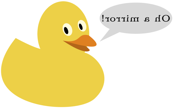
Figure 11.4 – A mirrored scope
\documentclass[tikz,border=10pt]{standalone}
\usepackage{tikzducks}
\begin{document}
\begin{tikzpicture}
  \begin{scope}[xscale=-1,transform shape]
    \duck[laughing,speech={\tiny Oh a mirror!}]
  \end{scope}
\end{tikzpicture}
\end{document}
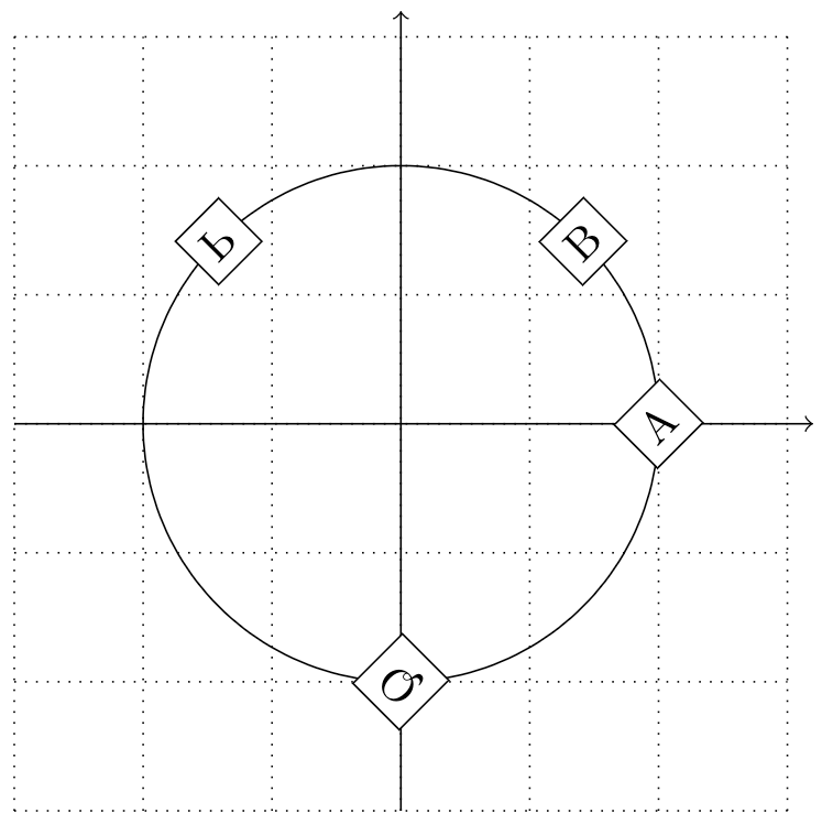
Figure 11.5 – Multiple transformations of nodes
\documentclass[tikz,border=10pt]{standalone}
\usepackage{tikzducks}
\begin{document}
\begin{tikzpicture}[transform shape, every node/.style={draw, fill=white}]
  \draw[thin,dotted] (-3,-3) grid (3,3);
  \draw[->] (-3,0) -- (3.2,0);
  \draw[->] (0,-3) -- (0,3.2);
  \draw circle(2);
  \node[xshift=2cm, rotate=45] {A};
  \node[rotate=45, xshift=2cm] {B};
  \node[rotate=45, yshift=2cm, yscale=-1] {P};
  \node[yscale=-1, yshift=2cm, rotate=45] {Q};
\end{tikzpicture}
\end{document}
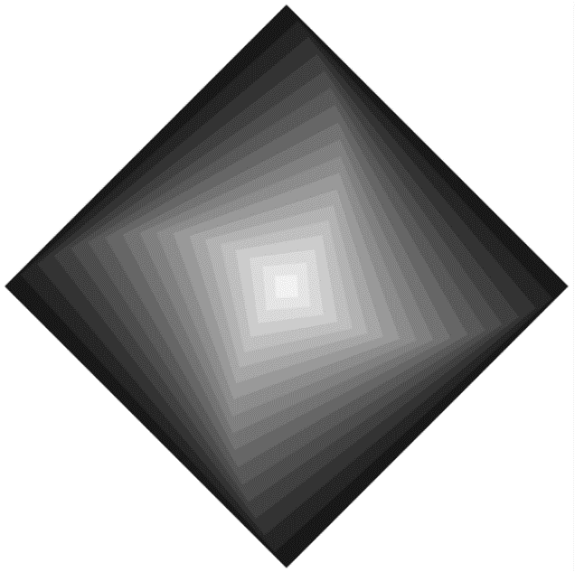
Figure 11.6 – Rotated and scaled squares
\documentclass[tikz,border=10pt]{standalone}
\usetikzlibrary{positioning}
\begin{document}
\begin{tikzpicture}
  \foreach \i in {90,85,...,5}
    \node[fill=black!\i, scale=\i, rotate=\i/2] {};
\end{tikzpicture}
\end{document}
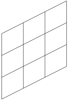
Figure 11.7 – A slanted 3×3 grid
\documentclass[tikz,border=10pt]{standalone}
\usetikzlibrary{positioning}
\begin{document}
\begin{tikzpicture}
%  \draw[thin,dotted] (-3,-3) grid (3,3);
%  \draw[->] (-3,0) -- (3,0);
%  \draw[->] (0,-3) -- (0,3);
  \draw[yslant=0.5] (0,0) grid +(3,3);
\end{tikzpicture}
\end{document}
Testing slanting
\documentclass[tikz,border=10pt]{standalone}
\usetikzlibrary{calc}
\begin{document}
\begin{tikzpicture}
  \draw[thin,dotted] (-1,-1) grid (3,3);
  \draw[->] (-1,0) -- (3.2,0);
  \draw[->] (0,-1) -- (0,3.2);
  \filldraw[yslant=1] (0,0) circle (0.3) node [right] {1}
    (1,0) circle (0.3) node [right] {2}
    (1,0) circle (0.3) node [right] {3}
    (3,0) circle (0.3) node [right] {4}
    (0,1) circle (0.3) node [right] {5}
   ;
\end{tikzpicture}
\end{document}
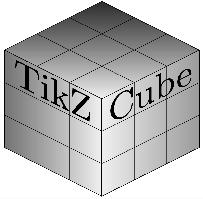
Figure 11.8 – A cube made from slanted grids
\documentclass[tikz,border=10pt]{standalone}
\usetikzlibrary{positioning}
\begin{document}
\begin{tikzpicture}
  \draw[yslant=0.5,
    left color=gray!10, right color=gray!70]
    (3,-3) rectangle +(3,3)
    (3,-3)   grid    +(3,3);
  \draw[yslant=-0.5,
    left color=black!50, right color=gray!10]
    (0,0) rectangle +(3,3)
    (0,0) grid +(3,3);
  \draw[yslant=0.5,xslant=-1,
    bottom color=gray!10, top color=black!80]
    (3,0) rectangle +(3,3)
    (3,0) grid +(3,3);
  \node[yslant=-0.5, scale=3.2]
    at (1.5,1.75) {TikZ};
  \node[yslant= 0.5, scale=3.2]
    at (4.5,1.75) {Cube};
\end{tikzpicture}
\end{document}
Transformations without effect
\documentclass[border=10pt]{standalone}
\usepackage{tikz}
\usetikzlibrary{positioning}
\begin{document}
\begin{tikzpicture}
  \node (tex) [fill=orange, text=white] {TEX};
  \node (pdf) [fill={rgb:red,244;green,15;blue,2},
    text=white, right=of tex] {PDF};
  \draw (tex) edge[->,yshift= 0.1mm, rotate= 4] (pdf);
  \draw (tex) edge[->,yshift=-0.1mm, rotate=-4] (pdf);
\end{tikzpicture}
\end{document}

Figure 11.9 – Transformed arrows
\documentclass[border=10pt]{standalone}
\usepackage{tikz}
\usetikzlibrary{positioning}
\begin{document}
\begin{tikzpicture}
  \node (tex) [fill=orange, text=white] {TEX};
  \node (pdf) [fill={rgb:red,244;green,15;blue,2},
    text=white, right=of tex] {PDF};
  \draw (tex) edge[->,transform canvas={yshift= 0.1mm,rotate=4}] (pdf);
  \draw (tex) edge[->,transform canvas={yshift=-0.1mm,rotate=-4}] (pdf);
\end{tikzpicture}
\end{document}
Please rate (and possibly review) the book on Amazon if you got it there, your feedback means much to me and helps to get an extended second edition!
Go to next chapter.