Here are the Code examples of this chapter. These pages are currently being updated over time (adding pictures, captions, and possibly further examples). Visit again soon for updates. Of course, the best way to use this page is together with the book for getting the explanations.
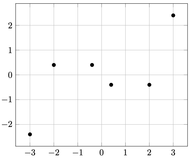
Figure 13.1 – Plotting coordinates
\documentclass[tikz,border=10pt]{standalone}
\usepackage{pgfplots}
\pgfplotsset{compat=1.18}
\begin{document}
\begin{tikzpicture}
  \begin{axis}[grid]
    \addplot[only marks] coordinates
      { (-3,-2.4)  (-2,0.4) (-0.4,0.4)
        (0.4,-0.4) (2,-0.4) (3,2.4) };
  \end{axis}
\end{tikzpicture}
\end{document}
Plotting with classic TikZ
\documentclass[tikz,border=10pt]{standalone}
\begin{document}
\begin{tikzpicture}
  \draw[->] (-3,0) -- (3,0);
  \draw[->] (0,-3) -- (0,3);
  \foreach \i in {-3,-2,-1,1,2,3} {
    \node at (\i,-0.2) {\i};
    \node at (-0.2,\i) {\i};
  }
  \draw[domain=-3:3, samples=50, thick] plot (\x, \x^3/5 - \x);
\end{tikzpicture}
\end{document}
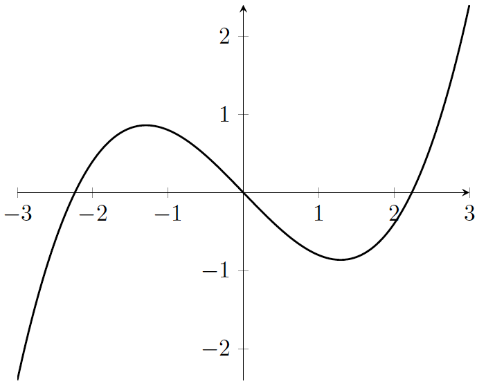
Figure 13.2 – A cubic plot with a centered x-axis and y-axis
\documentclass[tikz,border=10pt]{standalone}
\usepackage{pgfplots}
\begin{document}
\begin{tikzpicture}
  \begin{axis}[axis lines=center]
    \addplot[samples=80, smooth, thick, domain=-3:3]
      {x^3/5 - x};
  \end{axis}
\end{tikzpicture}
\end{document}
Defining a plot style
\documentclass[tikz,border=10pt]{standalone}
\usepackage{pgfplots}
\pgfplotsset{every axis plot post/.append style =
  {samples=80, smooth, thick, black, mark=none} }
\begin{document}
\begin{tikzpicture}
  \begin{axis}[axis lines = center, domain = -3:3]
    \addplot {x^3/5 - x};
  \end{axis}
\end{tikzpicture}
\end{document}
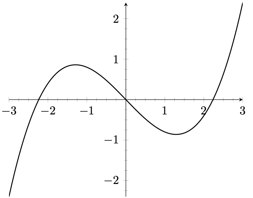
Figure 13.3 – Axes with minor ticks
\documentclass[tikz,border=10pt]{standalone}
\usepackage{pgfplots}
\begin{document}
\begin{tikzpicture}
  \begin{axis}[axis lines=center, minor tick num=3]
    \addplot[samples=80, smooth, thick, domain=-3:3]
      {x^3/5 - x};
  \end{axis}
\end{tikzpicture}
\end{document}
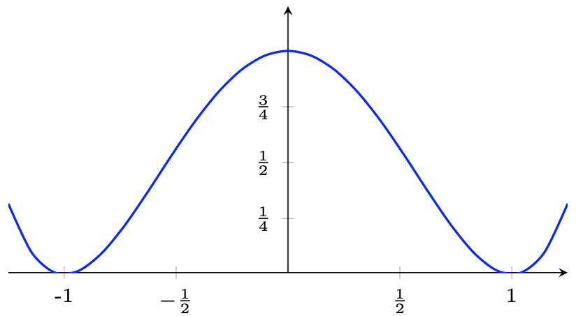
Figure 13.4 – Customized ticks
\documentclass[tikz,border=10pt]{standalone}
\usepackage{pgfplots}
\pgfplotsset{every axis plot post/.append style={thick,smooth,mark=none}}
\begin{document}
\begin{tikzpicture}
  \begin{axis}[axis lines = middle, axis equal image,
    domain = -1.25:1.25, y domain = 0:1.25,
    ymax = 1.2,
    tick label style = {font=\scriptsize},
    xtick = {-1, -0.5, 0.5, 1},
    xticklabels = {-1, $-\frac{1}{2}$, $\frac{1}{2}$, 1},
    ytick = {0.25, 0.5, 0.75},
    yticklabels = {$\frac{1}{4}$, $\frac{1}{2}$,
    $\frac{3}{4}$} ]
  \addplot { (x^2-1)^2 };
\end{axis}
\end{tikzpicture}
\end{document}
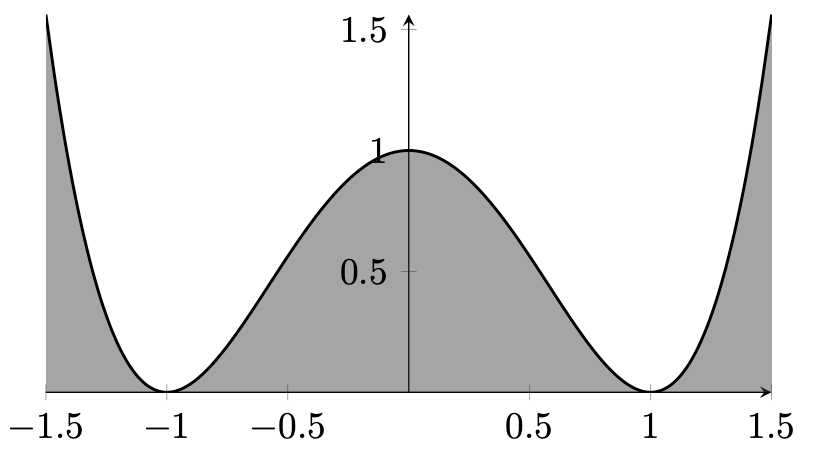
Figure 13.5 – Filling an area below a plot
\documentclass[tikz,border=10pt]{standalone}
\usepackage{pgfplots}
\usepgfplotslibrary{fillbetween}
\pgfplotsset{every axis plot post/.append style =
  {samples=80, smooth, thick, black, mark=none} }
\begin{document}
\begin{tikzpicture}
\begin{axis}[axis lines = center,
  axis equal image, domain = -1.5:1.5]
  \addplot[name path=quartic] {(x^2-1)^2};
  \path[name path=xaxis] (axis cs:-1.6,0)
    -- (axis cs:1.6,0);
  \addplot[darkgray, opacity=0.5]
    fill between[of=quartic and xaxis];
\end{axis}
\end{tikzpicture}
\end{document}
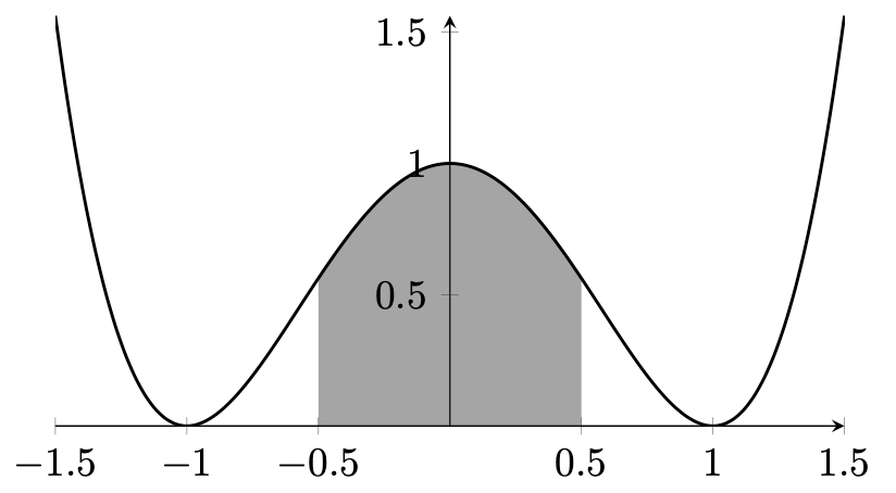
Figure 13.6 – Filling a segment below a plot
\documentclass[tikz,border=10pt]{standalone}
\usepackage{pgfplots}
\usepgfplotslibrary{fillbetween}
\pgfplotsset{every axis plot post/.append style =
  {samples=80, smooth, thick, black, mark=none} }
\begin{document}
\begin{tikzpicture}
\begin{axis}[axis lines = center,
  axis equal image, domain = -1.5:1.5]
  \addplot[name path=quartic] {(x^2-1)^2};
  \path[name path=xaxis] (axis cs:-1.6,0)
    -- (axis cs:1.6,0);
  \addplot[darkgray, opacity=0.5]
    fill between[of=quartic and xaxis,
    soft clip = {domain=-0.5:0.5} ];
\end{axis}
\end{tikzpicture}
\end{document}
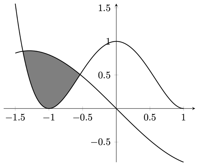
Figure 13.7 – Filling an area between plots
\documentclass[tikz,border=10pt]{standalone}
\usepackage{pgfplots}
\usepgfplotslibrary{fillbetween}
\pgfplotsset{every axis plot post/.append style =
  {samples=80, smooth, thick, black, mark=none} }
\begin{document}
\begin{tikzpicture}
  \begin{axis}[axis lines = center, axis equal,
      domain = -1.5:1]
    \addplot[name path=cubic]   {x^3/5 - x};
    \addplot[name path=quartic] {(x^2-1)^2};
    \addplot fill between[of=cubic and quartic, split,
      every segment/.style      = {transparent},
      every segment no 1/.style = {gray, opaque}];
  \end{axis}
\end{tikzpicture}
\end{document}
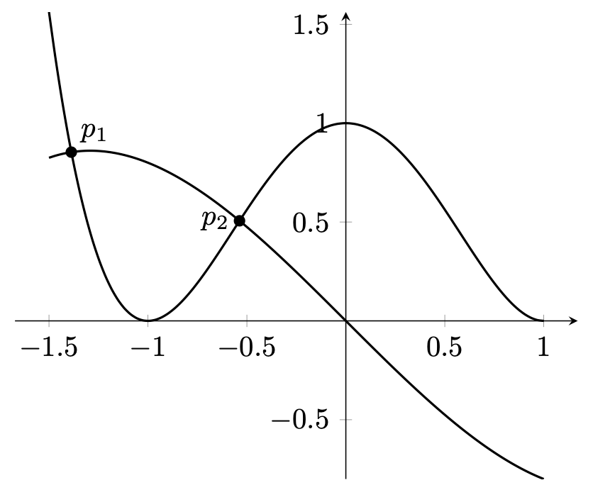
Figure 13.8 – Intersection points of plots
\documentclass[border=10pt]{standalone}
\usepackage{pgfplots}
\usetikzlibrary{intersections}
\pgfplotsset{every axis plot post/.append style =
  {samples=80, smooth, thick, black, mark=none} }
\begin{document}
\begin{tikzpicture}
  \begin{axis}[axis lines = center, axis equal,
      domain = -1.5:1]
    \addplot[name path=cubic]   {x^3/5 - x};
    \addplot[name path=quartic] {(x^2-1)^2};
    \fill[name intersections = {of=cubic and quartic,
     name=p}]
      (p-1) circle (2pt) node [above right] {$p_1$}
      (p-2) circle (2pt) node [left]        {$p_2$};
\end{axis}
\end{tikzpicture}
\end{document}
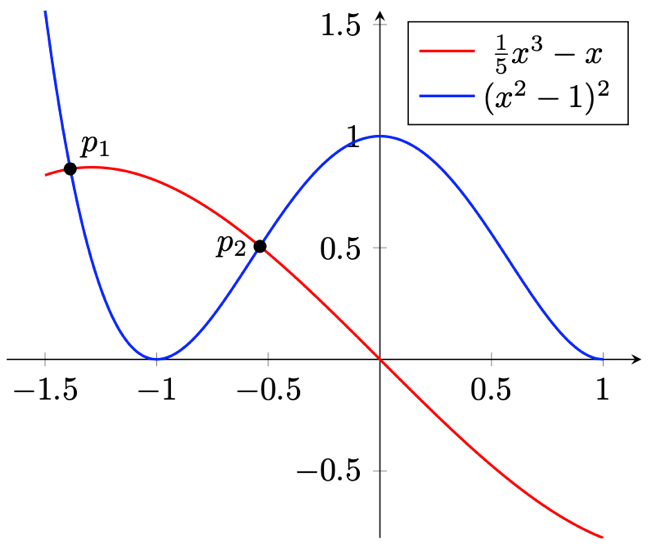
Figure 13.9 – Plots with a legend
\documentclass[border=10pt]{standalone}
\usepackage{pgfplots}
\usetikzlibrary{intersections}
\pgfplotsset{every axis plot post/.append style =
  {samples=80, smooth, thick, mark=none} }
\begin{document}
\begin{tikzpicture}
  \begin{axis}[axis lines = center, axis equal,
      domain = -1.5:1,
      legend entries = {$\frac{1}{5}x^3-x$, $(x^2-1)^2$}]
    \addplot[red,  name path=cubic] {x^3/5 - x};
    \addplot[blue, name path=quartic] {(x^2-1)^2};
    \fill[name intersections = {of=cubic and quartic,
     name=p}]
      (p-1) circle (2pt) node [above right] {$p_1$}
      (p-2) circle (2pt) node [left]        {$p_2$};
  \end{axis}
\end{tikzpicture}
\end{document}
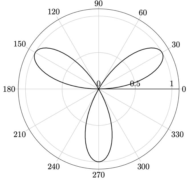
Figure 13.10 – A trigonometric function in a polar coordinate system
\documentclass[border=10pt]{standalone}
\usepackage{pgfplots}
\usepgfplotslibrary{polar}
\begin{document}
\begin{tikzpicture}
\begin{polaraxis}
  \addplot[domain=0:180, samples=100, thick] {sin(3*x)};
\end{polaraxis}
\end{tikzpicture}
\end{document}
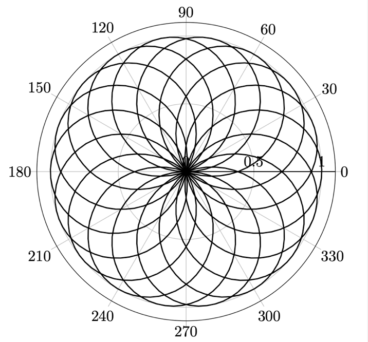
Figure 13.11 – A trigonometric function over multiple times 360 degrees
\documentclass[border=10pt]{standalone}
\usepackage{pgfplots}
\usepgfplotslibrary{polar}
\begin{document}
\begin{tikzpicture}
\begin{polaraxis}
  \addplot[domain=0:2880, samples=800, thick] {sin(9*x/8)};
\end{polaraxis}
\end{tikzpicture}
\end{document}
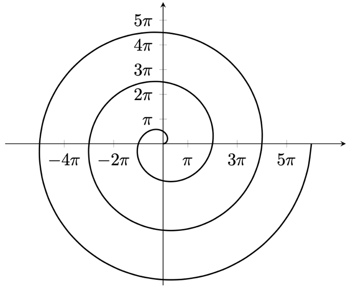
Figure 13.12 – Archimedean Spiral
\documentclass[border=10pt]{standalone}
\usepackage{pgfplots}
\pgfplotsset{trig format plots=rad}
\begin{document}
\begin{tikzpicture}
  \begin{axis}[axis lines = middle, axis equal,
      domain = 0:6*pi, ymin=-18, ymax=18,
      xtick = {-4*pi,-2*pi,pi,3*pi,5*pi},
      ytick = {pi, 2*pi, 3*pi, 4*pi, 5*pi},
      xticklabels = {$-4\pi$, $-2\pi$,
        $\vphantom{1}\pi$, $3\pi$, $5\pi$},
      yticklabels = {$\vphantom{1}\pi$, $2\pi$,
        $3\pi$, $4\pi$, $5\pi$}
    ]
    \addplot[samples=120, smooth, thick, variable=t]
      ( {t*cos(t)}, {t*sin(t)} );
\end{axis}
\end{tikzpicture}
\end{document}
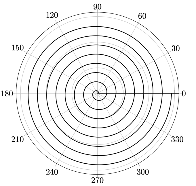
Figure 13.13 – Archimedean Spiral in a polar coordinate system
\documentclass[border=10pt]{standalone}
\usepackage{pgfplots}
\pgfplotsset{compat=1.18}
\usepgfplotslibrary{polar}
\begin{document}
\begin{tikzpicture}
  \begin{polaraxis}[yticklabel=\empty]
    \addplot[domain=0:2880, samples=200, smooth, thick] {x};
  \end{polaraxis}
\end{tikzpicture}
\end{document}
With radian angles:
\documentclass[border=10pt]{standalone}
\usepackage{pgfplots}
\pgfplotsset{compat=1.18}
\usepgfplotslibrary{polar}
\begin{document}
\begin{tikzpicture}
  \begin{polaraxis}[yticklabel=\empty]
    \addplot[domain=0:16*pi, samples=400, smooth, thick,
      data cs=polarrad] {x};
  \end{polaraxis}
\end{tikzpicture}
\end{document}
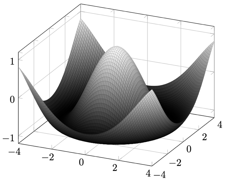
Figure 13.14 – A plot in 3D coordinates
\documentclass[border=10pt]{standalone}
\usepackage{pgfplots}
\usepgfplotslibrary{colormaps}
\pgfplotsset{trig format plots=rad}
\begin{document}
\begin{tikzpicture}
  \begin{axis}[
      domain    = -4:4, samples    = 70,
      y domain  = -4:4, samples y  = 70,
      colormap/blackwhite, grid]
    \addplot3[surf] { cos(sqrt(x^2+y^2)) };
  \end{axis}
\end{tikzpicture}
\end{document}
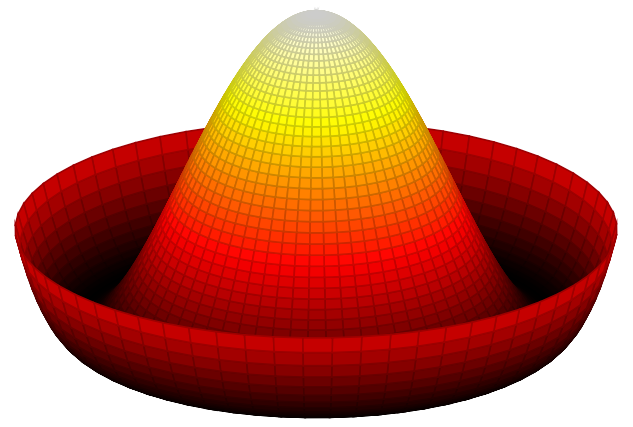
Figure 13.15 – A sombrero plot
\documentclass[tikz,border=10pt]{standalone}
\usepackage{pgfplots}
\usepgfplotslibrary{colormaps}
\begin{document}
  \begin{tikzpicture}
    \begin{axis}[hide axis, colormap/hot2]
      \addplot3 [surf, z buffer=sort, trig format plots=rad,
        samples=65, domain=-pi:pi, y domain=0:1.25,
        variable=t, variable y=r]
        ({r*sin(t)}, {r*cos(t)}, {(r^2-1)^2});
    \end{axis}
  \end{tikzpicture}
\end{document}
Please rate (and possibly review) the book on Amazon if you got it there, your feedback means much to me and helps to get an extended second edition!
Go to next chapter.
Here I found how this can be plotted with gnuplot: Mexican hat potential polar.svg from Spontaneous symmetry breaking (Sombrero potential) at Wikipedia.